Practical Frameworks
Almost no application builds an inverted index from scratch. The mechanics of the previous sections, postings, merges, ranking, compression, are already implemented, tuned, and battle-tested in libraries and database engines. The engineering choice is which one to adopt, and that choice follows the quality, latency, and storage tradeoff from the chapter opener. This section covers two ready-to-use options: full-text search inside a relational database, and the Lucene library. The distributed engines built on Lucene are the subject of the next section.
Full-text search in your database
If an application already stores its documents in a relational database, the simplest option is often to search them there. PostgreSQL offers full-text search as a built-in feature, and SQLite provides a similar capability through its FTS5 module. There is no separate service to run and no index to keep synchronized with the source data.
PostgreSQL models text search with two data types. A tsvector is a document reduced to a sorted set of normalized lexemes, produced by to_tsvector, which tokenizes the text, removes stop words, and applies stemming through a configurable dictionary. A tsquery is a search expression with Boolean operators and phrase constraints, produced by to_tsquery. The match operator @@ tests whether a tsvector satisfies a tsquery.
The speed comes from a GIN index, which stands for Generalized Inverted Index and is a genuine inverted index in the sense of this chapter. GIN stores a set of (key, posting list) pairs, where each key is a lexeme and its posting list holds the row identifiers of the documents that contain it. The lexemes themselves are organized in a B-tree so a lookup is fast, and posting lists are stored compressed; a lexeme with very many rows is promoted from a flat posting list to its own B-tree of row identifiers. A multi-word query resolves each lexeme to its posting list and intersects them, the same sorted-postings merge we saw in the first section. To keep inserts cheap, GIN can buffer new entries in a pending list and merge them into the main structure later, trading a little query overhead for faster writes.
Because a tsvector column and a GIN index live inside the database, full-text predicates combine naturally with ordinary SQL: a single query can match text, filter on other columns, join related tables, and run inside a transaction. The following example shows the full pattern, from schema to ranked search with a predicate:
-- 1. Define a table for movies
CREATE TABLE movies (
  id        SERIAL PRIMARY KEY,
  title     TEXT NOT NULL,
  overview  TEXT NOT NULL,
  rating    REAL,
  year      INT,
  tsv       tsvector
);

-- 2. Populate the tsvector column for full-text search
--    'A' = highest weight (title gets more influence)
--    'B' = lower weight (overview contributes less)
UPDATE movies
SET tsv = setweight(to_tsvector(title), 'A') ||
          setweight(to_tsvector(overview), 'B');

-- Create a GIN index for fast lookup
CREATE INDEX movies_tsv_idx ON movies USING GIN(tsv);

-- 3. Search with ranking and a predicate on year
SELECT id, title, year,
       ts_rank(tsv, to_tsquery('Star & Wars')) AS r
FROM movies
WHERE tsv @@ to_tsquery('Star & Wars')
  AND year < 2000
ORDER BY r DESC
LIMIT 10;
Step 2 builds the inverted index: to_tsvector tokenizes, normalizes, and stems the text, and setweight assigns one of four weight labels (A through D) so that ts_rank can weight matches differently by field; here title matches (weight A) count more than overview matches (weight B). Step 3 combines term matching (@@), a metadata predicate (year < 2000), and frequency-based ranking (ts_rank) in a single query. The database evaluates the GIN index lookup and the year filter together and chooses an efficient execution plan.
Where PostgreSQL needs a running server, SQLite embeds the entire database in a single file with no separate process, which makes its FTS5 module the lightest full-text option of all. FTS5 stores a genuine inverted index behind a virtual table and, unlike PostgreSQL’s ts_rank, ranks with true BM25 through a built-in bm25() function. Creating the index, loading documents, and running a ranked query take only a few statements:
-- Virtual table backed by an FTS5 inverted index (Porter stemming)
CREATE VIRTUAL TABLE books USING fts5(title, author, tokenize = 'porter unicode61');

-- Load documents (one row per book)
INSERT INTO books (title, author) VALUES ('Database Systems', 'Garcia-Molina');

-- Ranked search: MATCH selects candidates, bm25() scores them
SELECT title, bm25(books) AS score
FROM books
WHERE books MATCH 'database systems'
ORDER BY score;   -- bm25() is negative, so ascending puts the best match first
The MATCH operator accepts the same Boolean and phrase syntax as a dedicated engine, and because the score is true BM25, the ranking lines up with the hand-rolled BM25 of the previous section. SQLite FTS5 is a common choice for on-device and application-embedded search, where running a server alongside the app is not an option.
For collections up to a few million documents on a database you already operate, this is often all the search infrastructure an application needs. Conceptually, one could even build the inverted index by hand as an ordinary table of (term, document, frequency) rows with a B-tree index on the term column; the hands-on notebook does exactly this to make the structure concrete.
Lucene
Apache Lucene, created by Doug Cutting in 1999 and an Apache project since 2001, is the open-source Java library at the core of most production search platforms. It provides the full toolkit of this chapter: analysis, inverted indexing, term weighting, and ranking. Figure 1 shows how its pieces fit together. The current major version is Lucene 10 (10.5 as of mid-2026). Major releases change APIs; in particular, Lucene 10 removed the convenience searcher.doc() method (use reader.storedFields() instead) and requires an explicit Field.Store argument when constructing numeric fields. The concepts below are stable across versions; the hands-on notebook uses the Lucene 10 API.
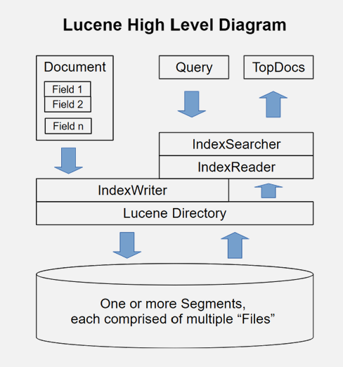
Figure 1:Lucene’s architecture: the write path (Document, IndexWriter, Directory, Segments) and the read path (Query, IndexSearcher, IndexReader, Directory, Segments, TopDocs) meet at the Directory storage abstraction.
Documents, fields, and analyzers
Lucene models a document as a set of named fields, and not every document needs every field. A field carries a name, a value, and a type that specifies whether the value is tokenized, what is written to the inverted index, and whether the original value is stored for retrieval. These three choices are independent: a long body field is typically tokenized and indexed for search but not stored, so the application fetches the original text from its own database. Field subclasses cover the common cases: a text field is tokenized and indexed with term frequencies and positions; string and numeric fields are indexed without tokenization for exact-match and range queries on metadata; a stored-only field is kept but not searchable.
Fields are indexed independently. If both a title field and a body field contain “house”, Lucene treats the two occurrences as distinct terms, internally prefixed as “title:house” and “body:house”. This is what lets a search weight a title match more heavily than a body match, or apply different normalization to each field.
Tokenization is the job of an analyzer, and the choice of analyzer must be identical for indexing and for querying. The standard analyzer lowercases and strips punctuation; the English analyzer additionally removes stop words and applies a Porter stemmer; custom analyzers can combine filters such as stemming, length limits, and case handling. Changing the analyzer means rebuilding the index.
// Comparing analyzer output for the same text
var text = "I think text's values' color goes here; WHAT happens ...";

// StandardAnalyzer: lowercase, strip punctuation, keep possessives
print_tokens(new StandardAnalyzer(), text);
// -> i think text's values color goes here what happens ...

// EnglishAnalyzer: + stop-word removal + Porter stemming
print_tokens(new EnglishAnalyzer(), text);
// -> think text valu color goe here what happen ...

// Custom stop words
var stopWords = new CharArraySet(Arrays.asList("i", "do"), false);
print_tokens(new EnglishAnalyzer(stopWords), text);
// -> think text valu color goe here what happen ...
Segments and updates
Lucene writes the index as a set of immutable segments. Each time an IndexWriter flushes, it creates a new segment, which reduces contention and protects against corruption. Because segments are immutable, Lucene never edits a document in place, and it has no primary key: internally a document is known only by a docId that can change when segments merge. Deletes and updates therefore identify documents by content. A delete-by-term marks every document whose chosen key field holds a given value, for example id:"B-10432", by flipping a bit in the segment’s live-documents list rather than erasing any data; a delete-by-query does the same for documents matching an arbitrary query. An update is a delete-by-term of the key value followed by an add of the new version, applied atomically. A configurable merge policy periodically combines smaller segments into larger ones, and only during a merge are the documents flagged as deleted physically dropped. Searching runs over all live segments in parallel and merges their results, which is the seed of the distributed scaling in the next section.
The following shows how documents are built and added to an index:
// Set up analyzer, directory, and writer
Analyzer analyzer = new EnglishAnalyzer();
Directory directory = FSDirectory.open(Paths.get("./index"));
IndexWriter writer = new IndexWriter(directory, new IndexWriterConfig(analyzer));

// Build a document from application data
Document doc = new Document();
doc.add(new TextField("title", "Star Wars", Field.Store.YES));
doc.add(new IntField("year", 1977, Field.Store.YES));
doc.add(new TextField("body", "A long time ago ...", Field.Store.NO));
writer.addDocument(doc);

// Close the writer to flush a new segment
writer.close();
Each TextField is tokenized and indexed; the IntField supports exact and range queries on metadata. Setting Store.NO on the body means its text is searchable but not retrievable from results, keeping the stored-fields footprint small.
Querying and scoring
A search uses an IndexSearcher over the index directory, usually with a query parser that turns user input into a query and applies the same analyzer used at indexing time. Results come back as a TopDocs object holding the best-scoring documents and their scores. Beyond plain keyword queries, Lucene supports field-scoped terms with boosts (a title match weighted higher), range queries, wildcards, and fuzzy matching within an edit distance. Queries can also be built programmatically, combining clauses that must, should, or must-not match, or that only filter without affecting the score.
Lucene ranks with BM25 by default, computed per field so that the document frequency and length normalization use that field’s statistics. Each query clause contributes a per-term score, and the document’s final score is their sum:
Here is the contribution of one query term (or clause), and clauses marked as filters contribute zero.
This is the BM25 of the previous section with two practical additions: a per-clause boost factor, and the Lucene IDF variant with the extra 1 inside the logarithm that keeps the weight positive even for very common terms. Lucene also applies one optimization: it leaves out the constant factor in the numerator. That factor is the same for every document, so it only rescales the scores by a constant and cannot change their order; ignoring it saves work without affecting the ranking. Lucene’s raw scores therefore come out smaller (roughly half at the default ) than the formula above, while the order stays the same. A helpful diagnostic, explain, prints how each clause contributed to a document’s score, which is invaluable when tuning boosts and field weights.
// Set up a searcher and a multi-field query parser
IndexSearcher searcher = new IndexSearcher(DirectoryReader.open(directory));
QueryParser parser = new MultiFieldQueryParser(
    new String[]{"title", "body"}, analyzer);

// Simple keyword query (searches title and body, ranked by BM25)
Query q = parser.parse("star wars");
TopDocs results = searcher.search(q, 10);

// Access stored fields (Lucene 10 API)
StoredFields storedFields = searcher.getIndexReader().storedFields();
for (ScoreDoc hit : results.scoreDocs) {
    Document d = storedFields.document(hit.doc);
    System.out.printf("%.2f  %s (%s)\n", hit.score,
        d.get("title"), d.get("year"));
}

// Programmatic query with filter, boost, and explain
Query query = new BooleanQuery.Builder()
    .add(IntField.newRangeQuery("year", 1950, 2000), Occur.FILTER)
    .add(new TermQuery(new Term("title", "shawshank")), Occur.MUST)
    .add(new BoostQuery(
        new TermQuery(new Term("body", "hope")), 1.5f), Occur.SHOULD)
    .build();

TopDocs top = searcher.search(query, 10);
// Score breakdown for the top hit
System.out.println(searcher.explain(query, top.scoreDocs[0].doc));
The explain output decomposes the score into each clause’s contribution, showing the IDF, TF, field length, boost, and normalization parameters. For the query above, it might look like this:
7.4038 = sum of:
  0.0 = match on required clause, product of:
    0.0 = # clause
    1.0 = year:[1950 TO 2000]           // FILTER: must match, no score
  1.0 = year:[1990 TO 2000]             // SHOULD: contributes 1.0
  3.0980 = weight(title:shawshank in 0) [BM25Similarity], result of:
    3.0980 = score(freq=1.0), computed as boost * idf * tf from:
      6.5023 = idf, computed as log(1 + (N - n + 0.5) / (n + 0.5)) from:
        1 = n, number of documents containing term
        999 = N, total number of documents with field
      0.4765 = tf, computed as freq / (freq + k1 * (1 - b + b * dl / avgdl)) from:
        1.0 = freq, occurrences of term within document
        1.2 = k1, term saturation parameter
        0.75 = b, length normalization parameter
        2.0 = dl, length of field
        2.2533 = avgdl, average length of field
  3.3057 = weight(body:hope in 0) [BM25Similarity], result of:
    3.3057 = score(freq=1.0), computed as boost * idf * tf from:
      1.5 = boost                       // the BoostQuery factor
      4.7687 = idf, computed as log(1 + (N - n + 0.5) / (n + 0.5)) from:
        8 = n, number of documents containing term
        1000 = N, total number of documents with field
      0.4621 = tf, computed as freq / (freq + k1 * (1 - b + b * dl / avgdl)) from:
        1.0 = freq, occurrences of term within document
        1.2 = k1, term saturation parameter
        0.75 = b, length normalization parameter
        8.0 = dl, length of field
        8.335 = avgdl, average length of field
Every quantity from the BM25 formula is visible: the IDF with its log(1 + ...) variant, the saturating TF with k1, b, dl, and avgdl, and the boost factor. Filter clauses contribute zero to the score but must still be satisfied. This makes it possible to diagnose why a document ranks where it does and to tune field boosts accordingly.
Higher-level pipelines
Above these engines sit frameworks that orchestrate retrieval as one step in a larger pipeline, combining keyword search with dense retrieval, rerankers, and language-model generation. Haystack is a widely used example. Because these frameworks belong to the retrieval-augmented generation setting, we cover them in a later chapter on retrieval-augmented generation rather than here.