Inverted Files
Consider a tiny collection of three documents:
: “The cat sat on the mat”
: “The dog chased the cat”
: “The cat and the dog played”
A query for “cat” should return , , and ; a query for “dog” should return and . With three documents we could simply read each one and check. With three million documents we cannot. We need a structure that takes us straight from a query term to the documents that contain it, without touching the rest of the collection. That structure is the inverted index, and this section explains why it makes query cost depend on the query rather than on the size of the collection.
Why scanning does not scale
Recall from Classical Text Retrieval that a document is represented as a sparse vector over the vocabulary. Assume a collection of documents and a vocabulary of terms. On average a document contains distinct terms, with much smaller than , and a typical query contains about terms, with much smaller than (five query terms is a common figure).
The most direct storage scheme reserves one entry for every term in every document: entries in total. In the set-of-words model each entry is a single bit that records whether the term occurs; the bag-of-words model stores a term frequency instead. Almost all of these entries are zero, because each document uses only a small fraction of the vocabulary. Storing the full matrix is therefore wasteful, and a sparse layout that keeps only the non-zero entries per document reduces storage from to entries.
The sparse layout saves space, but it does not save time. To answer a query we still scan every document, and for each one we read terms that the query never asked about. Here we rely on a property of the classical models: Boolean retrieval, the vector space model, and BM25 all score a document from its query terms alone, under the assumption that terms contribute independently. Only the entries for the query terms affect the result, so almost everything we read is discarded. This is exactly the property the inverted index will exploit.
This property is what makes classical retrieval fast, and it is also its limit. It does not hold for dense retrieval, which we cover in a later chapter on semantic search, where a document’s relevance depends on its whole embedding rather than on the presence of individual query terms. A dense system cannot restrict its attention to a handful of postings, which is why classical lexical retrieval remains orders of magnitude faster than dense retrieval and why the two are often combined.
Inverting the layout
Since only the query terms matter, we can organize storage around terms instead of documents. Rather than storing, for each document, the list of terms it contains, we store, for each term, the list of documents that contain it. This is the inverted index, also called the inverted file. Each term points to a postings list: the document identifiers in which the term appears. Figure 1 shows the inverted index for the three-document collection above.
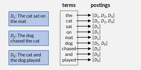
Figure 1:An inverted index over a three-document collection: each term in the vocabulary points to its postings list.
Inverting the layout does not change how much we store. There are still term-document pairs. What changes is how much we read per query. A query touches only the postings lists of its query terms. If the pairs are spread over terms, an average postings list holds entries, so a query of terms reads about entries instead of all .
The read cost is proportional to , so inverted files scale linearly with the collection: double the documents and both the index and the average read roughly double. For small to large collections this is comfortable. The book and code indexes, under a gigabyte and around a gigabyte and a half, fit entirely in memory on one machine, so a query with a few keywords is answered almost instantly. The average-term assumption behind those reads often overstates the cost here, because someone searching a book catalog is usually after a specific title and types rare, discriminative words whose postings lists are shorter than average. Under practical conditions, inverted files work very well across this whole range.
The trouble is common words. Stop words and other high-frequency terms have postings lists far longer than average, and they are what makes large collections expensive. On the book and code collections they are a nuisance rather than a blocker: we can drop stop words from the query, searching “Lord of the Rings” as “lord” and “ring” while ignoring “of” and “the”, and lean on the rare, discriminative terms. At web scale the same query behaves differently. A stop word on half of 10 billion pages carries roughly 19 GB of postings on its own, and even after dropping it, “lord” and “ring” each occur in hundreds of millions of pages, some close to 1 GB of postings apiece. No amount of stop-word removal rescues a plain postings scan when the discriminative terms are themselves frequent.
The web index also no longer fits on one machine at more than 20 TB, so it lives mostly on disk and must be distributed. Inverted files degrade gracefully rather than suddenly, remaining practical across a wide range of sizes, but the combination of an enormous collection and unavoidably frequent terms is what eventually breaks the simple scheme. Keeping web-scale queries fast despite gigabyte postings lists is the job of the additional strategies we return to later: skip pointers and early termination, pruned and tiered indexes, caching, the sharding, and scaling out.
Query length is a cost lever in the same way, which matters for query expansion. Expanding a query, introduced in Advanced Text Processing, adds related terms to raise recall, but every added term is another postings list to read and merge, and the extra terms add noise that can lower precision. On a large collection, where a single frequent term can already cost gigabytes, expansion has to be weighed against query cost, not against precision alone.
The structure of the index
An inverted index has three parts. The vocabulary (or dictionary) holds the distinct terms and serves as the lookup key. Each term points to its postings list. A separate document table stores per-document metadata, such as a title, author, or URL, that the ranker and the result page need but that is not itself searched term by term.
The two tables below make this concrete, using book titles from the library collection we return to throughout the chapter. The document table records one row per document, keyed by an integer identifier:
| ID | Title | Author | Year |
|---|---|---|---|
| 1 | Database Systems: The Complete Book | Garcia-Molina, Ullman, Widom | 2008 |
| 2 | Pattern Recognition and Machine Learning | Christopher Bishop | 2006 |
| 3 | Data Science from Scratch | Joel Grus | 2015 |
| 4 | Operating System Concepts | Silberschatz, Galvin, Gagne | 2018 |
| 5 | Artificial Intelligence: A Modern Approach | Russell, Norvig | 2020 |
| ... | ... | ... | ... |
| 50 | Frankenstein | Mary Shelley | 1818 |
The inverted index maps each term in those titles to the sorted list of document identifiers where it occurs:
| Term | Postings (document IDs) |
|---|---|
computer | [9, 10, 12, 14] |
design | [8, 9] |
introduction | [7, 15] |
software | [9, 13] |
systems | [1, 14] |
the | [1, 7, 8, 9, 13, 16, 19, 20, 26, 28, 31, 32, 35, 38, 43, 47] |
| ... | ... |
The row for term the illustrates the earlier point about common words: even in a 50-title collection, the stop word “the” has a longer postings list than any content term.
For Boolean retrieval over the set-of-words model, the postings lists need only the document identifiers; term frequencies and document frequencies are not required. As documents are added, their identifiers are appended to the postings of the terms they contain. When documents arrive in order, each postings list stays sorted by increasing document identifier. That sorted order is not incidental: it is what makes the evaluation below efficient.
Boolean retrieval over postings
A Boolean query combines terms with AND, OR, and NOT. Because each postings list is a set of document identifiers, the operators map directly onto set operations:
expr1 AND expr2: the intersection of the two postings sets.expr1 OR expr2: the union of the two postings sets.expr1 AND NOT expr2: the set difference, the documents ofexpr1that are not inexpr2.
Nesting AND and OR combines these operations, and the same rules generalize to more than two operands. The NOT operator needs care. We never materialize NOT expr2 on its own, because its complement can contain almost the whole collection. A pure negation, or an OR with a negated operand such as “cat OR NOT dog”, would force us to enumerate millions of identifiers. Such a query is also rarely what a user means: “cat OR NOT dog” selects every document except those that contain “dog” but not “cat”. We therefore allow NOT only inside an AND that has at least one non-negated operand, and we apply the negated parts last, as a subtraction from the candidates found so far.
In code this is remarkably direct: an inverted index is a dictionary from terms to postings sets, and the Boolean operators are the language’s own set operators. Taking an artifical example collection:
cat   = index['cat']    # [4, 5, 12, 13, 14, 15, 20, 22, 30, 34]
dog   = index['dog']    # [1, 3, 4, 6, 9, 10, 13, 21, 22, 23, 29, 30]
horse = index['horse']  # [6, 10, 11, 14]
bird  = index['bird']   # [2, 3, 8, 15, 26, 35, 36]

cat & dog      # cat AND dog       -> [4, 13, 22, 30]
horse | bird   # horse OR bird     -> [2, 3, 6, 8, 10, 11, 14, 15, 26, 35, 36]
cat - dog      # cat AND NOT dog   -> [5, 12, 14, 15, 20, 34]

# Queries nest freely, because each operation returns another set of IDs:
(cat & dog) | ((horse & cat) - bird)   # (cat AND dog) OR (horse AND cat AND NOT bird)
                                       #   -> [4, 13, 14, 22, 30]
(cat | dog) & (horse | bird)           # (cat OR dog) AND (horse OR bird)
                                       #   -> [3, 6, 10, 14, 15]
(cat | dog) - (horse | bird)           # (cat OR dog) AND NOT (horse OR bird)
                                       #   -> [1, 4, 5, 9, 12, 13, 20, 21, 22, 23, 29, 30, 34]
The last two lines show the permitted use of NOT: negation applied to the result of an AND, never on its own. This set-based version is clear but reads every full postings list into memory. The next step scales it down.
Merging sorted postings as streams
Loading whole postings lists into memory does not scale to lists with millions of entries. Instead we read them as sorted streams and merge them, advancing one entry at a time, much like merging sorted lists. Suppose the postings are:
cat: 1, 4, 10
dog: 3, 4, 8, 10, 12
To evaluate “cat AND dog” we look at the head of each stream and always advance the smaller one. When both heads are equal, that document satisfies the AND, so we emit it and advance both streams.
| cat head | dog head | comparison | action | output |
|---|---|---|---|---|
| 1 | 3 | 1 < 3 | advance cat | |
| 4 | 3 | 4 > 3 | advance dog | |
| 4 | 4 | equal | emit, advance both | 4 |
| 10 | 8 | 10 > 8 | advance dog | |
| 10 | 10 | equal | emit, advance both | 10 |
| exhausted | 12 | cat empty | stop |
The result is the sorted list 4, 10. The merge stops as soon as one stream is exhausted: once cat runs out, no later document can match, even though dog still has the entry 12.
The other operators follow the same pattern with a different emit rule. For “cat OR dog” we emit the smaller head at each step and advance the stream it came from, producing the union 1, 3, 4, 8, 10, 12. For “cat AND NOT dog” we emit a cat entry only when it is strictly smaller than the current dog head, producing 1. Because every operator consumes sorted streams and emits a sorted stream, the operators compose: the output of one merge feeds directly into the next.
The whole scheme depends on the postings being sorted, and we get that ordering for free as long as we only ever append documents with increasing identifiers: a new document’s identifier is larger than any already in a list, so it simply goes at the end. Deletions and updates would break this. Removing a document leaves a gap, and changing one alters its terms, so the tidy append-only order no longer holds without rewriting postings lists in place. Many systems avoid that cost by refusing in-place edits. Lucene, for example, treats its index as append-only: every new document is assigned the next identifier and is never modified afterwards, a deletion only flips a marker in a per-segment list of live documents so that the document is filtered out of results, and an update is a delete-by-term, which removes whatever document matches a chosen key term such as a unique identifier, followed by a fresh insert. Documents flagged as deleted are physically removed only later, in bulk, when segments are merged, which we revisit in Practical Frameworks. This design has a valuable side effect. Because existing postings are effectively static, writers and readers barely need to coordinate: new documents are flushed into new segments while queries keep running against the existing ones, so the postings a reader is scanning never shift underneath it.
From matching to ranking
Boolean evaluation answers a yes-or-no question: does a document satisfy the query? It produces a candidate set, but no order within it. For anything beyond exact filtering we want the best documents first, which means scoring each candidate. That splits retrieval into two stages: a retriever that uses the inverted index to gather candidates, and a ranker that scores them. The next section shows how the ranked models from Chapter 1, the binary independence model, the vector space model, and BM25, all run over the same postings lists.