Query Understanding
The first three sections closed the recall gap on the document side. A well-processed collection now has one token per concept, phrases identified, and compounds split. The chapter opener’s other failure remains: the query “Bücher von Goethe” arrives as three tokens and the retriever has no idea that “Bücher” and “books” are the same concept, that “Goethe” names a person, or that the sentence is a request for works by a specific author. This section adds three tools that extract that kind of structure from free-text: word-relationship expansion, part-of-speech tagging, and named entity recognition. The section ends with the practical concern of spelling: a query that arrives misspelled needs to be repaired before any of these tools can help.
Word relationships: synonyms and homonyms
Stemming and lemmatization collapse different surface forms of the same word onto one token. They do nothing about the looser assumption we used so far: that one normalized token is independent of another normalized token. Every retrieval model in the book to this point has relied on it, treating tokens as unrelated dimensions with no notion that two of them might mean similar things or that one might mean two things. Real language breaks that assumption in two directions. A synonym is two different words for the same concept (“buy” and “purchase”); a homonym is one word carrying two concepts (“bank” the institution and “bank” the riverside). Lemmatization helps with neither, because “buy” and “purchase” reduce to unrelated stems and “bank” keeps a single stem whichever sense is meant. This section handles both with classical lexical tools; the semantic search chapter returns to the independence assumption in full and replaces it with learned representations that place related tokens near each other.
Synonyms break recall. A user searching a product catalog for “purchase history” misses documents indexed under “buy” or “buying”, even though they hold exactly what the user wants, purely because the tokens differ. Two responses:
Synonym expansion (classical). Attach a synonym list to each token. When the document contains “purchase”, also index “buy” and “acquire”. When the query contains “buy”, also search for “purchase” and “acquire”. The synonym lists come from curated resources (WordNet for English, thesaurus databases for other languages) or from domain-specific glossaries (medical terminologies, legal dictionaries).
Dense embeddings (modern). Instead of maintaining synonym lists, learn a vector space where “buy” and “purchase” naturally end up near each other. This is the approach of the semantic search chapter and it subsumes the synonym problem, at the cost of an embedding model and a vector index.
Domain vocabularies show the same problem more sharply. The chapter opener’s F1 query, “Who won the F1 race on the weekend?”, needs to match documents that call the same event a “Grand Prix” and never use the tokens “F1” or “race” at all. WordNet does not capture this mapping because it is not a linguistic synonym but a domain shorthand. The fix is a domain-specific synonym list maintained by the search team: F1 maps to {Formula 1, Formula One, Grand Prix}, race maps to {Grand Prix, GP}. Product-search systems maintain similar lists for brand aliases (“iPhone” -> “Apple iPhone”, “iPhones”) and category synonyms (“laptop” -> “notebook”).
Hand-maintained lists work well for the common, high-value terms a search team can anticipate, but they cannot keep up with the long tail: driver names the list has never seen, one-off event aliases, or code words specific to a community. This is where dense retrieval starts to pay for itself, because an embedding model learns which words appear in similar contexts without any manual list. Modern production stacks combine both: hand-crafted lists for the head, embeddings for the tail. The full argument comes back in the semantic search chapter.
Homonyms are the other direction, and the harder one. A query for “bank” cannot know whether the user means the financial institution or the riverside, and “lead” could be the metal or the verb meaning to guide. Two responses again:
Context from surrounding words (classical). The words around a homonym usually fix its sense. Part-of-speech tagging is the simplest case: “lead” the noun (the metal) and “lead” the verb (to guide) carry different tags, so tagging at index and query time separates them. Broader lexical context helps further: a text that also mentions “money”, “account”, or “loan” points to the financial “bank”, while “river”, “water”, or “shore” points to the riverside. This works whenever there is enough surrounding text to read.
Contextual embeddings (modern). Sentence encoders and large language models represent a word by the company it keeps, so “bank” in “the river bank” and “bank” in “the savings bank” receive different vectors. They resolve the sense from context without any hand-written rules, which is why they handle homonyms far more reliably than lexical rules do. This is the approach developed in the semantic search chapter.
Both approaches lean on context, so both fail when the query is too short to supply any: a bare query “bank” gives the system nothing to disambiguate on. There the only options are to return results for both senses or to ask, which is what web search does with “did you mean” suggestions. Genuine ambiguity with no context is inherent to language, and no technique fully removes it.
Hypernyms and hyponyms
WordNet provides two more relationships that expand queries in a different direction. A hypernym is a broader category (“animal” is a hypernym of “cat”), and a hyponym is a narrower one (“cat” is a hyponym of “animal”, and “mammal” is both a hyponym of “animal” and a hypernym of “cat”). These relationships form a hierarchy, and every English noun in WordNet sits somewhere in that hierarchy.
Three retrieval uses:
Faceted search. A user searching for “animals” is offered “cats”, “dogs”, “birds” as sub-facets that drill down into the hypernym tree. If the initial query returns too few results, the user is offered the parent facet (“mammals”) that broadens it. Amazon’s category tree and Wikipedia’s category system are both hypernym hierarchies dressed up as navigation UIs.
Query expansion with weighted hyponyms. A search for “cat” is silently expanded to include hyponyms like “kitten”, “tabby”, “siamese”, each with a lower weight than the original term. Documents about specific cat breeds surface for a general “cat” query.
Relevance ranking with hypernym paths. Instead of expanding the query, the scoring function is adjusted so a document mentioning “labrador” contributes something to a query for “dog” even without an explicit expansion.
from nltk.corpus import wordnet

for synset in wordnet.synsets('cat', pos='n')[:3]:
    print(synset.name(), '->', synset.definition())
    print('  hypernyms:', [h.name() for h in synset.hypernyms()])
    print('  hyponyms: ', [h.name() for h in synset.hyponyms()[:3]])

# cat.n.01 -> feline mammal usually having thick soft fur and no ability to roar
#   hypernyms: ['feline.n.01']
#   hyponyms:  ['domestic_cat.n.01', 'wildcat.n.03']
WordNet covers English; multilingual equivalents such as Open Multilingual WordNet exist for around 30 languages but with less coverage than the English version.
Part-of-speech tagging
Sentences are made of words that fall into grammatical classes: noun, verb, adjective, adverb, pronoun, article, and so on. A part-of-speech tagger assigns one of these labels to each token in a sentence, using surrounding words to disambiguate cases where the same surface form belongs to different classes (“run” as a noun in “a good run” versus “run” as a verb in “I run daily”). Figure 1 shows a POS-tagged parse tree for a simple English sentence, with the POS tags at the leaves and phrase-level structure above them.
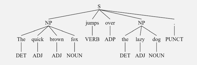
Figure 1:Constituency parse tree for “The quick brown fox jumps over the lazy dog.” POS tags (DET, ADJ, NOUN, VERB, ADP, PUNCT) appear at the leaves; phrase-level constituents such as NP (noun phrase) sit at intermediate nodes.
POS tagging supports three retrieval-side uses:
Selective stop-word filtering. Not every occurrence of “it” is a pronoun. In the phrase “the IT department”, “IT” is a noun and should be kept; in “it is easy”, it should be dropped. POS-aware stop-word filtering keeps content-bearing occurrences and removes function-word ones. This is how the “IT security” case from the stop-word discussion in the previous section is handled correctly.
Lemmatizer disambiguation. WordNet’s lemmatizer needs the POS tag:
wordnet.lemmatize("meeting", "n")returns"meeting"whilewordnet.lemmatize("meeting", "v")returns"meet". Feeding the lemmatizer the wrong tag produces the wrong lemma.Question-form analysis. The query “Who is Albert Einstein?” has a WH-word (“who”), a copula verb (“is”), and a proper noun (“Albert Einstein”). Combining that structure with the recognition that “Albert Einstein” is a person’s name (see the next subsection) tells the retriever this is a person-lookup query, and the right response is not a keyword search but a lookup in a people database or a redirect to Wikipedia. The intent-routing section returns to this example.
Three families of taggers have been used historically:
Rule-based taggers apply hand-written rules based on suffixes and surrounding words. Fast and simple, but each language needs its own rule set and rules cannot easily be extended.
Statistical (HMM) taggers model the sentence as a sequence of hidden POS states emitting observed tokens. Transition and emission probabilities are learned from a POS-tagged corpus; decoding uses the Viterbi algorithm. Dominant approach from the 1990s to the mid-2010s.
Neural taggers run a small transformer or LSTM over the token sequence and output a POS tag per token. This is the current default in
spaCyand in most Hugging Face pipelines.
All three families reach around 97-99% accuracy on English news text. On informal genres (social media, product reviews) the neural taggers pull ahead because they handle out-of-vocabulary words better.
import spacy
nlp = spacy.load('en_core_web_sm')

doc = nlp("Who is Albert Einstein?")
for token in doc:
    print(f"{token.text:12s} {token.pos_:8s} {token.tag_:6s} {token.dep_}")

# Who          PRON     WP     nsubj
# is           AUX      VBZ    ROOT
# Albert       PROPN    NNP    compound
# Einstein     PROPN    NNP    attr
# ?            PUNCT    .      punct
Two tag sets appear in practice. The pos_ field uses the coarse Universal tag set (around 17 categories: NOUN, VERB, ADJ, ADV, PROPN, PRON, DET, ADP, ...). The tag_ field uses the fine-grained Penn Treebank tag set (around 45 categories: VBZ for third-person singular verb, NNP for proper noun, WP for WH-pronoun). The Universal tags are enough for retrieval-side filtering; the Penn tags are needed for building parse trees.
Named entity recognition
The tokens “Albert Einstein” in the previous example are not just two proper nouns; they name a specific person, and the retrieval system that recognizes them as such can act on that recognition. Named entity recognition (NER) classifies spans of tokens into entity types: person, location, organization, product, date, money, and so on. NER is a natural extension of POS tagging: it runs after tokenization and POS tagging (or jointly with them in modern neural pipelines) and outputs entity spans.
The approaches behind NER mirror the POS taggers above. The earliest systems were rule-based, combining gazetteers (lists of known people, places, and organizations) with hand-written patterns such as a capitalized word following a title like “Dr.” or preceding a suffix like “Inc.”. Statistical sequence models replaced them: a conditional random field (CRF) labels each token from features of the token and its neighbours, trained on annotated corpora such as CoNLL-2003. Modern systems fine-tune a transformer for token classification, tagging each sub-word with its entity type. This is the current state of the art and what spaCy’s larger models and Hugging Face NER pipelines use.
doc = nlp("Jack Higgins deposits £50,000 with BestBank in London.")
for ent in doc.ents:
    print(f"{ent.text:15s} {ent.label_}")

# Jack Higgins    PERSON
# £50,000         MONEY
# BestBank        ORG
# London          GPE
For query understanding, four categories dominate the retrieval-side use cases:
Person names. “Who is Albert Einstein?” should trigger a person-lookup: prioritize Wikipedia, IMDb, MusicBrainz, and other person-oriented sources rather than running a keyword search across the whole web.
Time and date. “Who won the F1 race last weekend?” contains a temporal expression. Retrieval should restrict to news articles from the past few days and rank recent items above older ones.
Locations. “What to do in Basel?” should prioritize regional content and augment the results with a map. The location is a hard filter, not just another keyword.
Product brands. “Where can I buy the latest iPhone?” should boost shopping and product-review pages, and can trigger a price-comparison widget.
Every NER category exposes a routing decision. The classifier and router are the subject of the next section; this section only extracts the entities themselves.
NER also generates candidate phrases automatically: consecutive tokens tagged as PERSON produce a bi-gram or tri-gram like “Albert Einstein” that should be indexed as a unit, exactly as in the previous section’s phrase-detection discussion. This is often faster and more targeted than PMI or LHR scoring over the whole corpus, because named entities are exactly the phrases that matter for entity-oriented search.
For tooling, spaCy and Stanza provide NER for many languages out of the box, nltk offers a lighter ne_chunk, and the Hugging Face token-classification pipeline exposes fine-tuned transformer models such as dslim/bert-base-NER. Beyond libraries, the major cloud providers offer NER as a managed API: Amazon Comprehend, Google Cloud Natural Language, and Azure AI Language all return typed entities (often alongside key phrases and relations) without training a model. This convenience is why they anchor many production document-processing pipelines, extracting parties and amounts from contracts, fields from invoices, or names and dates from scanned forms.
Chunking with rule-based grammars
For queries that do not fit neatly into a POS-plus-NER analysis, a lightweight chunker groups consecutive tokens matching a small grammar. The classic pattern is:
NP -> DET? ADJ* NOUNwhich matches a noun phrase like “a red car” or “the lazy dog”. Chunking gives the retriever access to noun-phrase-level tokens without running a full parser. nltk.RegexpParser implements this cheaply:
grammar = r"NP: {<DT>?<JJ>*<NN>}"
chunker = nltk.RegexpParser(grammar)
tree = chunker.parse(nltk.pos_tag(nltk.word_tokenize("a red car")))
More elaborate grammars produce dependency parses that connect the noun phrase “red car” to the adjective “red” that modifies it. Stanford CoreNLP and spaCy’s dependency parser produce these for free once POS tags are available. For most retrieval scenarios noun-phrase chunking is enough.
Spell correction and “did you mean?”
Every query understanding pipeline has to handle typos. A user typing “Bücher von Goehte” (transposed letters) gets no results if the retriever demands an exact string match on “Goethe”, regardless of how good the rest of the pipeline is. The classical response is a two-part strategy: correct at both indexing time and query time.
At indexing time, keep the original token but also add the auto-corrected form. A document containing the misspelling “Goehte” is indexed under both “Goehte” and “Goethe”, so users find it whether they type the correct or the incorrect spelling.
At query time, run the query through the spell-checker. If a token is not in the dictionary, offer corrections and either search all of them silently or ask “Did you mean ‘Goethe’?”. Modern search engines do both: they auto-run the corrected query and let the user click back to the original spelling if the correction was wrong.
Spell correction is especially tricky for names. “Britney” is often misspelled as “Britny”, “Brittney”, or “Britnee”, which argues for folding them all back to “Britney”. The catch is that several of these forms are themselves legitimate names that other people genuinely carry, so a single variant can be at once a typo of one name and the correct spelling of another. A spell-checker that rewrites every variant to one canonical “Britney” then merges distinct people and loses anyone who is really spelled the other way. This is the “did you mean Britney, or Britnie?” problem. The pragmatic compromise is to keep the original spelling in the index and, at query time, expand to the common variants rather than silently rewriting to a single form.
Two standard algorithms underpin classical spell correction:
Edit distance (Damerau-Levenshtein). Score candidate corrections by the minimum number of insertions, deletions, substitutions, and transpositions to reach the query. Widely used but slow to compute exhaustively; production systems restrict the candidate set with a phonetic prefilter or a small edit-radius trie.
Phonetic codes (Soundex, Metaphone). Reduce each word to a compact code that captures its rough pronunciation. Different spellings of the same-sounding word share a code and are candidates for one another. Essential for name variants that no edit-distance approach can handle.
Query expansion and query rewriting
Several of the transformations described so far share a family resemblance. Synonym mapping, hypernym expansion, spell correction, alias substitution, and temporal normalization all take the tokens the user typed and change them so the resulting query matches more of the collection. In the IR literature these transformations fall under two umbrella names:
Query expansion adds tokens to the original query without removing the ones the user typed. Synonym expansion, weighted-hyponym expansion, and adding all common spelling variants of a name to a query all fall here. The original query terms usually stay at full weight and the added terms come in at a lower weight, so a document that matches the user’s exact words still ranks above one that matches only via expansion.
Query rewriting transforms the query text itself, replacing or restructuring tokens. Spell correction (“Goehte” -> “Goethe”), alias substitution (“F1” -> “Formula 1”), temporal normalization (“last weekend” -> a date range), and compound splitting on the query side (“Wolkenkratzer” -> “Wolken”, “Kratzer”) are query rewrites. The rewritten query goes to the retriever; the original may or may not be preserved for logging.
The line between the two blurs in practice. A rewrite that adds tokens alongside the originals (F1 OR "Formula 1" OR "Grand Prix") is an expansion in disguise. An expansion that later drops the original terms in favour of the added ones is a rewrite. What matters is that the retriever sees a different query from the one the user typed, and both directions are standard tools.
This chapter has been building both throughout:
Section 1 — language detection informs both expansion (which stop-word and synonym list to use) and rewriting (which stemmer to apply). Case, Unicode, and accent normalization are rewrites at the character level.
Section 2 — stemming and lemmatization are rewrites at the token level (“carried” -> “carri” for Porter, “carried” -> “carry” for WordNet).
Section 3 — compound splitting rewrites one token into several on both the document side and the query side.
Section 4 — synonym and hypernym mappings are expansions; spell correction is a rewrite.
Section 5 — temporal normalization and domain-alias substitution are rewrites applied during intent routing.
Two techniques not covered here belong in the same family and are worth naming so students recognize them elsewhere:
Pseudo-relevance feedback, also called blind feedback. This is the relevance-feedback and query-expansion mechanism of the Binary Independence Model from Probabilistic Ranking and BM25, run without any user judgements. Instead of asking the user which results are relevant, it assumes the top- retrieved documents are relevant and applies the same term-discrimination weighting to choose expansion terms, the high-scoring terms like “woodland” in that chapter’s worked example. It is a retrieval-model technique rather than a text-processing one, which is why it belongs with vector-space and BM25 ranking.
LLM-based query rewriting. A language model reformulates the query. Common patterns include HyDE (write a plausible answer and search for that instead of the question), multi-query (generate several rewrites and union their results), and step-back prompting (generalize the query one level before searching). These belong to the retrieval-augmented generation chapter.
The chapter opener’s F1 query is a plain example of query rewriting. “Who won the F1 race on the weekend?” is rewritten by dropping the WH-pronoun “who” and the verb “won” as non-content, expanding “F1” and “race” to “Formula 1” and “Grand Prix”, and turning “the weekend” into a date range. What reaches the retriever is a scoped keyword query rather than a question, and the next section walks that rewrite through the full routing pipeline. Classical rewriting stops there: it can retrieve the right race-report page but cannot produce the short answer “Verstappen”. That last step needs a reader or generator to extract the answer from the retrieved text which is covered in a later chapter (retrieval-augmented generation).
Where this sits in modern retrieval
Every classical technique in this section still runs somewhere in a modern search stack. Web search engines apply POS tagging, NER, and spell correction to every query before any retrieval or ranking. Product-search systems for e-commerce use NER heavily to extract brand names, category constraints, and numerical facets (“under $50”). Enterprise search over document management systems relies on synonym expansion using domain-specific terminologies.
The one classical technique that dense embeddings largely subsume is synonym expansion: a well-trained embedding model puts “purchase” and “buy” near each other in vector space, so the query “purchase history” retrieves documents about “buying” without an explicit synonym list. Hypernym reasoning is partially learned but less reliably: an embedding model may or may not know that a labrador is a dog, depending on the training data. POS tagging, NER, and spell correction remain explicit steps even in fully neural pipelines because they produce structured outputs (tags, spans, corrected strings) that downstream systems can act on discretely. Large language models can substitute for all of them in a single prompt, but for high-throughput retrieval the classical stack is still cheaper by orders of magnitude.
The final section takes everything this section produces (language ID, POS tags, entities, corrections) and turns it into a routing decision: which backend should the query go to?