Probabilistic Ranking and BM25 - Multimedia Retrieval

The Vector Space Model ranks effectively, but its weighting and similarity measures are heuristic. Probabilistic retrieval asks a more direct question: given query $Q$ and document $D_i$ , how likely is the document to be relevant? The Binary Independence Model (BIR) develops this idea from binary term evidence. BM25 then retains its probabilistic term weighting while adding the term-frequency saturation and document-length normalization missing from BIR and vector-space scoring.

Binary Independence Model¶

The BIR model uses the same tokenized vocabulary as the previous models, but represents each query and document as a set of terms. It was formalized by Robertson and Spärck Jones; see Relevance Weighting of Search Terms in the Further Reading section of the chapter summary. A component is 1 when a term is present and 0 when it is absent. It assumes that terms contribute independently and that non-query terms occur equally often in relevant and non-relevant documents. Under these assumptions, only query terms present in a document affect its rank.

Let $R$ denote relevance and $NR$ non-relevance for query $Q$ . Ranking by the posterior odds

\frac{P(R\mid D_i,Q)}{P(NR\mid D_i,Q)}

(1)

is equivalent to ranking by the document evidence after query-dependent constants are removed. Define

r_j=P(d_{i,j}=1\mid R,Q), \qquad n_j=P(d_{i,j}=1\mid NR,Q).

(2)

The first probability measures how often term $t_j$ occurs in relevant documents; the second measures how often it occurs in non-relevant documents. The resulting score is additive, but several probability terms must cancel before we reach that form. The derivation below explains why only query terms present in the document remain.

From posterior odds to the BIR score (optional reading)

Bayes’ rule separates the posterior odds into prior odds and document evidence:

\frac{P(R\mid \mathbf{d}_i,Q)}{P(NR\mid \mathbf{d}_i,Q)} = \frac{P(R\mid Q)}{P(NR\mid Q)} \cdot \frac{P(\mathbf{d}_i\mid R,Q)}{P(\mathbf{d}_i\mid NR,Q)}.

(3)

The prior odds $P(R\mid Q)/P(NR\mid Q)$ are the same for every document considered for query $Q$ . They affect the numerical score but not the ranking. We can therefore focus on the likelihood ratio containing the document evidence.

Under the binary representation, each component satisfies $d_{i,j}\in\{0,1\}$ : it is 1 when document $D_i$ contains term $t_j$ and 0 otherwise. Combined with term independence, this makes the probability of the complete document vector a product of Bernoulli probabilities. The exponents select the appropriate case: $r_j^{d_{i,j}}$ contributes $r_j$ when the term is present, while $(1-r_j)^{1-d_{i,j}}$ contributes $1-r_j$ when it is absent.

P(\mathbf{d}_i\mid R,Q) = \prod_{j=1}^{M} r_j^{d_{i,j}}(1-r_j)^{1-d_{i,j}},

(4)

P(\mathbf{d}_i\mid NR,Q) = \prod_{j=1}^{M} n_j^{d_{i,j}}(1-n_j)^{1-d_{i,j}}.

(5)

Substituting these products into the odds and taking the logarithm turns multiplication into addition:

\log\frac{P(R\mid \mathbf{d}_i,Q)}{P(NR\mid \mathbf{d}_i,Q)} = \log\frac{P(R\mid Q)}{P(NR\mid Q)} + \sum_{j=1}^{M} \left[ d_{i,j}\log\frac{r_j}{n_j} +(1-d_{i,j})\log\frac{1-r_j}{1-n_j} \right].

(6)

For a term absent from the query, BIR assumes $r_j=n_j$ . Both logarithms then become zero, so every non-query term disappears. For a query term, we can rearrange its contribution as

\log\frac{1-r_j}{1-n_j} + d_{i,j}\log\frac{r_j(1-n_j)}{n_j(1-r_j)}.

(7)

The first part depends on the query but not on the document, so it is another constant that does not change the ranking. The second part contributes only when $d_{i,j}=1$ . After removing all ranking constants, the remaining coefficient is

c_j=\log\frac{r_j(1-n_j)}{n_j(1-r_j)},

(8)

which produces the additive BIR score below.

Relevance Feedback¶

Initial estimates. Before any relevance information is available, the system must produce a first ranking. BIR commonly assumes that every query term has an equal chance of occurring in a relevant document, $r_j=0.5$ . It estimates occurrence in non-relevant documents from the term’s document frequency in the complete collection:

r_j=0.5, \qquad n_j=\frac{\text{df}(t_j)+0.5}{N+1}.

(10)

These initial values produce the first $c_j$ weights and therefore the first result list.

Collecting feedback. The user can now mark retrieved documents as relevant or non-relevant, for example through like and dislike controls. These judgements provide a sample of both classes. Because $r_j$ is the probability that term $t_j$ occurs in a relevant document, we can estimate it by counting how many judged relevant documents contain the term. We estimate $n_j$ in the same way from the judged non-relevant documents.

Updating the estimates. Suppose the user has judged $K$ documents and marked $L$ of them as relevant. Let $k_j$ be the number of judged documents containing $t_j$ , and let $l_j$ be the number that both contain $t_j$ and are relevant. The relevant sample therefore contains $l_j$ occurrences among $L$ documents. The non-relevant sample contains $k_j-l_j$ occurrences among $K-L$ documents. Without smoothing, the corresponding estimates would be

r_j\approx\frac{l_j}{L}, \qquad n_j\approx\frac{k_j-l_j}{K-L}.

(11)

In practice, BIR adds pseudo-counts so that small samples do not produce probabilities of exactly 0 or 1:

r_j=\frac{l_j+0.5}{L+1}, \qquad n_j=\frac{k_j-l_j+0.5}{K-L+1}.

(12)

The updated probabilities produce new $c_j$ weights and a revised ranking. Further rounds of feedback can refine the estimates, although users may be unwilling to judge many results.

Example: Feedback and query expansion

Consider the query dog forest. Suppose all 12 documents are judged, and $D_1$ and $D_3$ are marked relevant, leaving the other 10 documents as the non-relevant sample. Both relevant documents contain “dog” and “forest”, so feedback first refines the weights of the original query terms:

Term	Relevant documents containing term	Non-relevant documents containing term	$r_j$	$n_j$	$c_j$
“dog”	2	4	0.833	0.409	1.977
“forest”	2	5	0.833	0.500	1.609

With these refined weights, a document containing both “dog” and “forest” scores $1.977+1.609=3.586$ , an improved estimate over the initial, feedback-free weights.

Feedback has a second, independent use: we can compute $c_j$ for terms that never appeared in the query, using the same relevant and non-relevant samples. This tells us which additional terms help separate relevant from non-relevant documents, without requiring the user to reformulate anything.

Term	Relevant documents containing term	Non-relevant documents containing term	$r_j$	$n_j$	$c_j$
“woodland”	2	2	0.833	0.227	2.833
“algorithms”	0	1	0.167	0.136	0.236
“cats”	0	2	0.167	0.227	-0.386

The three terms illustrate three distinct roles:

“woodland” has a high positive $c_j$ : both relevant documents contain it, and only a fifth of the non-relevant documents do. It is a strong candidate for query expansion. Adding it to the query raises $D_1$ and $D_3$ to 6.419 and gives lexical variants such as $D_2$ and $D_{11}$ positive evidence even though they contain neither “dog” nor “forest”.
“algorithms” has a $c_j$ close to zero: it occurs in only one document overall, and that document is not relevant. The sample is too small to say whether the term discriminates at all, so it is best discarded, the same treatment we give to stop words that occur everywhere.
“cats” has a negative $c_j$ : it occurs only in non-relevant documents, both of which are technical distractors about pets and animal classification rather than the woodland adventure the user wants. Note that “cats” is a distinct token from “cat”, which does appear in $D_1$ ; the tokenizer does not know they share a root, so the two counts are entirely independent. A negative weight can therefore help demote or eliminate documents that share surface vocabulary with the query but belong to the wrong sense.

In practice, an automatic query expansion step keeps terms with a strongly positive $c_j$ , drops terms near zero, and may use strongly negative terms to penalize rather than reward a document.

BIR marks a change in ambition, not only a change in formula. The Vector Space Model ranks by geometric heuristics that happen to work well; BIR instead tries to explain relevance from first principles, estimating how likely a document is to be relevant given its terms. It still represents documents as term vectors and still combines evidence with the same OR-like accumulation as VSM: any query term found in the document contributes its weight to the score. What changes is the meaning of that weight. Instead of a heuristic tf-idf product, $c_j$ estimates the independent contribution of each query term toward relevance, grounded in how often the term separates relevant from non-relevant documents.

The restrictive assumptions behind this first version, binary term presence, term independence, and no document-length effect, are not inherent to the probabilistic idea itself. They make BIR tractable, and later probabilistic models relax them one at a time. The 2-Poisson model, for instance, models within-document term frequency directly instead of treating term presence as binary, at the cost of a more complex parameter estimation problem; see Robertson and Walker’s Some Simple Effective Approximations to the 2-Poisson Model for Probabilistic Weighted Retrieval in the Further Reading section of the chapter summary. Probabilistic language models take yet another route, estimating the probability that a document’s language model would generate the query. The section below develops BM25, which keeps BIR’s additive, per-term structure but approximates the 2-Poisson model’s term-frequency behaviour with a simpler saturating function.

The feedback mechanism also has a practical limitation worth mentioning. A user who rates a first result list of 10 documents gives us a sample of size $K=10$ from which to estimate $r_j$ and $n_j$ , far too small to pin down these probabilities reliably, especially for terms that appear in only one or two of the judged documents. Larger judged samples would improve the estimates, but no user will realistically rate hundreds of documents to make search work. This tension between statistical need and user effort is a recurring theme in relevance feedback, not a flaw specific to BIR.

Okapi BM25¶

BM25 was developed at London’s City University by Stephen Robertson, Karen Spärck Jones, and colleagues as a practical approximation to the 2-Poisson model. It became the robust default for free-text retrieval that BIR itself never was. Robertson and Zaragoza’s The Probabilistic Relevance Framework: BM25 and Beyond, listed in the Further Reading section of the chapter summary, surveys the complete derivation and its later extensions.

Three Unresolved Issues¶

Before introducing the BM25 formula, it helps to see exactly what the two preceding models still get wrong. Each issue below reappears as a concrete design decision in BM25.

Vector-space scoring rewards repetition without limit. Recall the running query cat dog forest from the Vector Space Retrieval section. Its inner product already ranks $D_7$ (four occurrences of “dog”, score 2.773 for that term alone) above $D_9$ (one occurrence of each query term, contributing 0.693 for “dog” toward its combined score of 1.537), even though $D_9$ is the only document that mentions “cat”, “dog”, and “forest” together. If a document repeated “dog” twenty times instead of four, its score would climb to 13.863, growing linearly and without bound. A ranking function that rewards raw repetition this directly is vulnerable to keyword stuffing: an author can inflate a document’s score simply by repeating a term, regardless of whether the document is actually about that topic.

Raw term frequency ignores what “coverage” means for document length. A term occurring once in a 3-token document (such as $D_9$ ) is stronger evidence of relevance than the same term occurring once in a 20-token document, because in the short document, that one occurrence forms a much larger share of the content. TF-IDF and the inner product treat both occurrences identically. Relevance should depend on how much of the document is about the query term, not merely how many times it appears. To reward the same relevance signal, a longer document should need proportionally more occurrences of a term than a shorter one to reach the same score.

Binary presence throws away frequency information, but the idea behind $r_j$ and $n_j$ is worth keeping. BIR’s document evidence is either 0 or 1, so it cannot express that $D_7$ mentions “dog” four times while $D_3$ mentions it once. At the same time, BIR contributes something valuable: the idea that a term’s ranking weight should reflect how well that term distinguishes relevant from non-relevant documents, not just how rare it is in the collection overall. BM25 keeps this probabilistic idea but combines it with a real-valued term-frequency component.

Term-Frequency Saturation¶

BM25 replaces the raw count in the TF-IDF product with a bounded function of term frequency:

\widehat{\text{tf}}_{k_1}=\frac{\text{tf}(k_1+1)}{\text{tf}+k_1}, \qquad k_1>0.

(13)

The first occurrence contributes strongly; later occurrences add progressively less; the value never exceeds $k_1+1$ no matter how often the term repeats. This directly answers the spamming issue: repeating “dog” twenty times can no longer produce an unbounded score. Parameter $k_1$ controls how quickly the function saturates. Values between 1 and 2 are common, with $k_1=1.2$ used in the running example. Figure 1 contrasts linear, square-root, and saturating term-frequency weights.

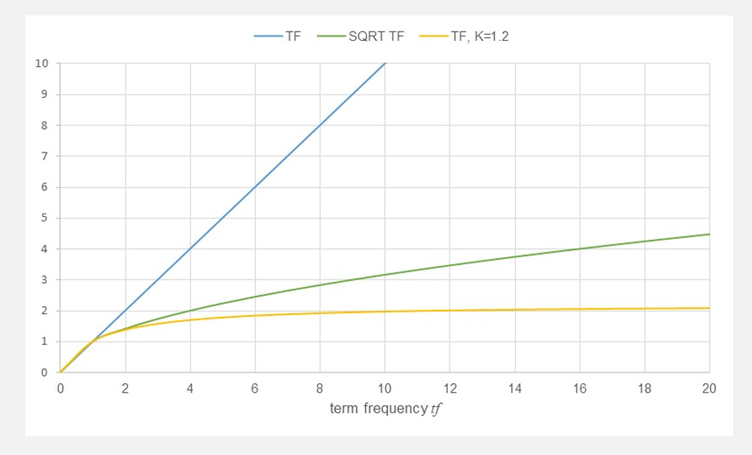
Figure 1:Linear, square-root, and BM25-saturated term-frequency weighting.

Document-Length Normalization¶

Saturation alone does not address the length issue: a document with tf=1 in 3 tokens and a document with tf=1 in 20 tokens still saturate identically. BM25 makes the saturation point depend on document length by scaling the denominator:

\widehat{\text{tf}}_{k_1,b}(D_i,t)=\frac{\text{tf}(D_i,t)(k_1+1)}{\text{tf}(D_i,t)+k_1\left(1-b+b\frac{|D_i|}{\text{avgdl}}\right)}.

(14)

Here $|D_i|$ is the number of processed tokens (=document length) and $\text{avgdl}$ is the collection’s average document length. For the running collection, $\text{avgdl}=9.67$ tokens. A single occurrence of “dog” in a 3-token document (shorter than average) contributes 1.393, while the same single occurrence in a 20-token document (longer than average) contributes only 0.696: the short document needs less repetition to reach the same weight because that occurrence covers a larger share of its content. Parameter $b\in[0,1]$ controls the strength of this effect: $b=0$ disables length normalization entirely, while $b=1$ applies the full length ratio. Figure 2 shows how the same term frequency receives more weight in a short document than in a long one.

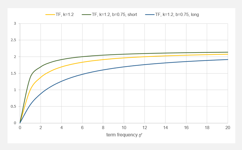
Figure 2:BM25 term-frequency saturation for average, short, and long documents.

Probabilistic IDF¶

The third issue was that BIR’s idea of estimating a term’s discriminating power from $r_j$ and $n_j$ is worth keeping even though its binary document model is not. Substituting the no-feedback BIR estimates ( $r_j=0.5$ and $n_j$ from document frequency) into the $c_j$ formula from the previous section gives exactly the classical BM25 weight:

\text{idf}_{\text{BM25}}(t)=\log\frac{N-\text{df}(t)+0.5}{\text{df}(t)+0.5}.

(15)

This value becomes negative when a term appears in more than half of the collection. Many implementations instead use the always-positive Lucene variant

\text{idf}_{+}(t)=\log\left(1+\frac{N-\text{df}(t)+0.5}{\text{df}(t)+0.5}\right)=\log\frac{N+1}{\text{df}(t)+0.5}.

(16)

Figure 3 compares these variants with the smoothed classical IDF introduced earlier. All encode the same core intuition that common terms provide less evidence, but their numerical values are not interchangeable.

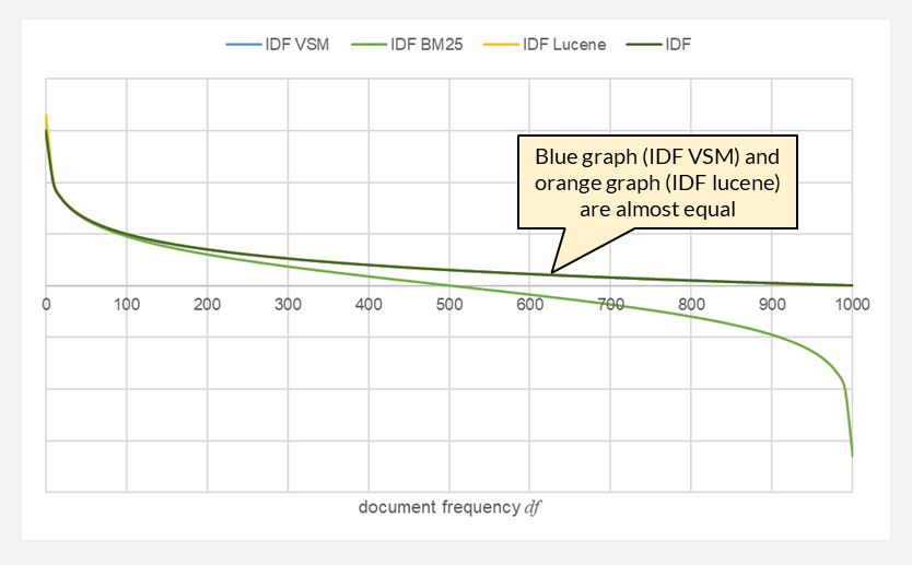
Figure 3:Classical, original BM25, and positive Lucene IDF variants.

A negative weight is undesirable for an additive scoring function: it would let a matching query term actively lower a document’s score, the opposite of what a match should do, and it complicates summing evidence across query terms of very different commonness. The Lucene weight $\log\frac{N+1}{\text{df}(t)+0.5}$ and the smoothed classical VSM weight $\log\frac{N}{\text{df}(t)}$ are nearly identical: comparing them shows that the Lucene variant is equal to the classical one exactly when $\text{df}(t)=N/2$ , slightly below it for rare terms, and slightly above it for common terms, never departing far in either direction. This is exactly the region where the original BM25 IDF turns negative, so Lucene’s variant tracks the familiar classical shape almost everywhere while staying non-negative where it matters. Lucene therefore adopts it as a numerically safer stand-in for the same underlying quantity rather than as a conceptually different weighting scheme.

Complete Formula and Running Example¶

Using the positive IDF variant gives the practical scoring function used in this example.

For $Q=$ cat dog forest, use $k_1=1.2$ , $b=0.75$ , and the same preprocessing as before. The 12 documents have $\text{avgdl}=9.67$ tokens. Their positive IDF values are 0.860 for “cat”, 0.693 for “dog”, and 0.550 for “forest”.

Example: BM25 ranking

Document	Length	TF (`cat`, `dog`, `forest`)	BM25 score
$D_9$	3	(1, 1, 1)	2.930
$D_1$	8	(2, 2, 1)	2.836
$D_{10}$	14	(2, 2, 2)	2.568
$D_{12}$	11	(1, 1, 0)	1.470
$D_3$	10	(0, 1, 1)	1.226
$D_7$	10	(0, 4, 0)	1.166
$D_4$	8	(1, 0, 0)	0.925
$D_8$	12	(0, 0, 4)	0.894
$D_5$	11	(0, 0, 2)	0.728
$D_6$	10	(0, 0, 1)	0.542

Documents $D_2$ and $D_{11}$ share no exact query term and score zero. The compact exact match $D_9$ ranks first, resolving the ordering that VSM’s inner product got wrong. Repetition keeps $D_1$ competitive, but saturation prevents the four occurrences of “dog” in $D_7$ from dominating the way it did under linear TF-IDF. Although $D_{10}$ repeats all three terms, its greater length lowers its score relative to $D_9$ : the same occurrences carry less weight once length normalization is applied.

Evaluation follows the same efficient pattern as vector-space retrieval. The system takes the union of the query-term posting lists, accumulates one BM25 contribution per matching term, and sorts candidates by decreasing score. Chapter 4 develops the posting-list algorithms used for this process.

Limitations and Modern Applications¶

BM25 remains lexical and bag-of-words based. It neither connects “cat” with “feline” nor distinguishes the natural and technical meanings of “forest”. It also assumes that document length should influence relevance in a consistent way, so $k_1$ and $b$ may require tuning for collections with unusual document types. Despite its probabilistic derivation, a BM25 score is a ranking value, not a calibrated probability of relevance.

Advantages: BM25 combines partial matching, discriminative term weighting, term-frequency saturation, and document-length normalization in an efficient additive score. It is transparent, fast, and difficult to improve upon as a lexical baseline.

Disadvantages: It retains lexical matching and term-independence assumptions, requires parameter choices, and does not directly represent phrase meaning or semantic similarity.

BM25 is the default or standard lexical ranker in systems built on Lucene, including Elasticsearch, Solr, and OpenSearch. It is also widely used as a first-stage retriever in retrieval-augmented generation and in hybrid search, where its exact lexical matches complement dense embedding retrieval.