From Text to Searchable Vectors
Retrieval models cannot operate directly on PDF files, HTML markup, or character streams. They compare structured representations of documents and queries. The feature extraction pipeline shown in Figure 1 creates these representations through five conceptual steps: extract text from the source format, split it into retrieval units, tokenize and normalize the text, construct a vocabulary, and summarize each unit as a feature vector. This produces two key artifacts:
Index - high-dimensional feature vectors for every retrieval unit, stored together with source metadata.
Vocabulary - the complete set of normalized terms used for both document and query processing.
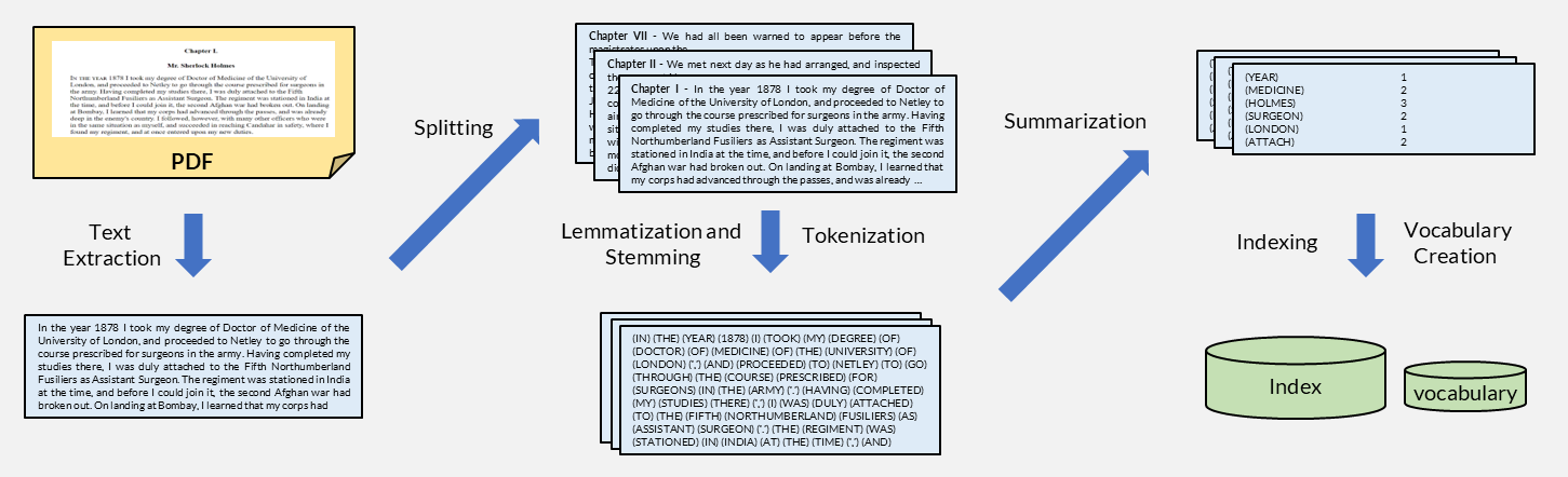
Figure 1:Text indexing pipeline: extract, split, tokenize, stem, summarize, then build the index and vocabulary.
Text Extraction
The first step extracts plain text and metadata from the source format. Documents arrive in many formats: PDF, EPUB, plain text, HTML, or office documents (DOCX, PPTX). Each format encodes content differently, mixing actual text with layout instructions, styling, and structural markup. The extraction step strips formatting and control sequences, isolates the character stream, and records metadata attributes (author, title, date) for later use in filtering.
Consider the HTML example in Figure 2. The header holds structured metadata (title, keywords) that can enrich the index entry, while the body contains the main text interleaved with markup tags. Extracting useful text from HTML requires parsing the DOM tree and distinguishing content nodes from navigation, scripts, and boilerplate. Although HTML follows a well-defined standard, real-world pages use diverse layouts, making robust extraction (often called scraping) a non-trivial engineering problem.
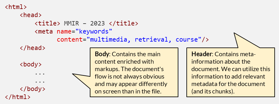
Figure 2:HTML document structure: metadata in the header, content in the body.
Source formats differ, so extraction normally relies on format-specific parsers and established libraries. The retrieval pipeline itself only requires that this stage return clean text and useful metadata; the implementation details can be selected for the collection at hand.
Source formats and extraction tools (optional reading)
Different source formats require different extraction strategies:
PDF: Text is stored as positioned glyphs, not logical paragraphs. Extraction must reconstruct reading order from coordinates. Tables and multi-column layouts are particularly challenging.
Office documents (DOCX, PPTX): ZIP archives containing XML. Libraries can parse the XML structure to extract text, but embedded images and charts require separate handling.
HTML/XML: Well-structured but noisy. Useful text must be separated from navigation menus, advertisements, and script blocks.
Plain text and Markdown: Minimal transformation needed, but encoding detection (UTF-8 vs. legacy encodings) and line-break conventions still require attention.
In practice, we rarely build extraction from scratch. Modern extraction pipelines rely on established libraries and frameworks:
Apache Tika: Java-based toolkit from the Apache Lucene ecosystem that auto-detects file types and extracts text and metadata from over 1,000 formats (PDF, DOCX, EPUB, email archives, images via OCR). Commonly used as the ingestion layer in Solr and Elasticsearch pipelines.
Unstructured (
unstructuredon PyPI): Open-source Python library designed for LLM/RAG pipelines. Handles PDFs, HTML, images, and office documents with built-in chunking support.MarkItDown (
markitdownon PyPI): Open-source Python library from Microsoft that converts PDF, DOCX, PPTX, XLSX, HTML, CSV, JSON, images, and audio into clean Markdown. Lightweight and popular for RAG preprocessing.Trafilatura: Focused on web content extraction. Strips boilerplate from HTML pages and returns clean article text.
PyMuPDF (fitz): Fast PDF text and layout extraction in Python, preserving reading order and table structure.
BeautifulSoup / lxml: HTML/XML parsers for custom extraction logic when off-the-shelf tools fall short.
The choice of extraction tool depends on the document mix in the collection, the required fidelity (do you need tables? images? footnotes?), and whether the pipeline must run at scale.
At this point, we must also decide on a character encoding for the index. UTF-8 is the dominant standard and handles virtually all scripts. Legacy collections may contain documents in older encodings (Latin-1, Shift-JIS) that require detection and conversion before indexing.
Splitting
As discussed in the previous section, retrieval granularity determines what constitutes a single retrieval unit. Once we have extracted the raw text from a document, we must split it into the units that will be indexed and returned to the user. In classical text retrieval, the splitting strategies are pragmatic and structure-driven:
By document boundary: Each file, email, or web page becomes one retrieval unit. This is the most common approach when documents are naturally self-contained.
By structural element: Books are split at chapter or section headings. Legal texts are split by article or paragraph number. The document’s own structure defines the boundaries.
By line or log entry: In observability systems like Elasticsearch, each log line becomes an independent retrieval unit. This enables searching millions of events by timestamp, severity, or content.
By fixed page or paragraph count: When no structural markup is available (e.g., scanned documents), we split at regular intervals such as every N paragraphs or every page.
These approaches share a common property: the splitting decision is made once during indexing and remains fixed. Each resulting unit is treated as an independent document by the retrieval models that follow. Figure 3 illustrates this for a novel split into chapter-sized retrieval units.
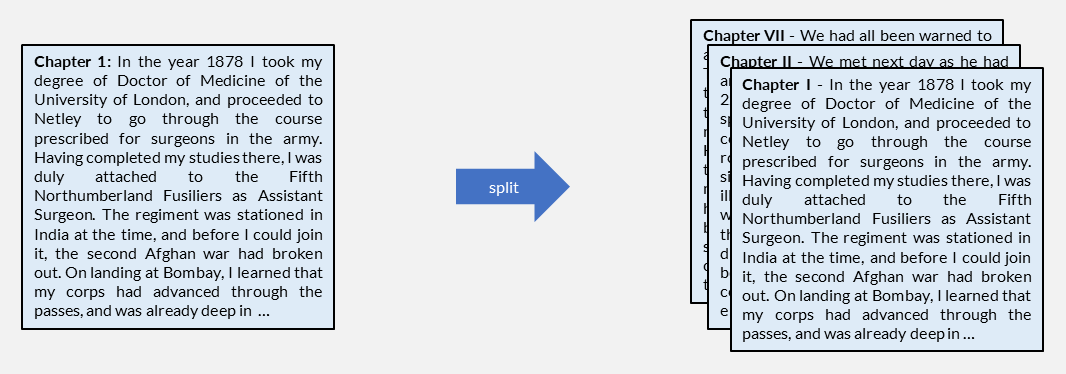
Figure 3:A single document divided into multiple smaller retrieval units.
Tokenization
Tokenization converts the extracted character stream into a sequence of discrete units called tokens. A token is an individual element in this sequence: it can be a word, a number, or a punctuation mark. A term is the normalized form of a token after processing (stemming, case folding). In classical text retrieval, tokens are typically whole words, and the two concepts are often used interchangeably. In later chapters, we will see that this equivalence breaks down when tokens become subword fragments or multi-word phrases.
For classical retrieval, we split text at whitespace and punctuation boundaries to produce word-level tokens. This requires decisions about edge cases: how to handle hyphenated words (“state-of-the-art”), numbers (“3.14”), abbreviations (“U.S.A.”), and possessives (“Watson’s”). In languages without explicit word boundaries (e.g., Japanese, Chinese), segmentation requires dictionary-based or statistical methods.
The most significant challenge is variation in word forms. Since retrieval models match documents to queries by comparing tokens, two tokens are either identical or unrelated. There is no notion of “almost the same”. A query for “cats” will not match a document containing only “cat” because these are distinct tokens. Similarly, “go”, “goes”, “went”, and “going” are four independent dimensions in the vocabulary despite sharing a meaning. The next subsection addresses this through stemming and lemmatization, which reduce inflected forms to a common token before indexing. Figure 4 shows the tokenization step applied to a document collection.
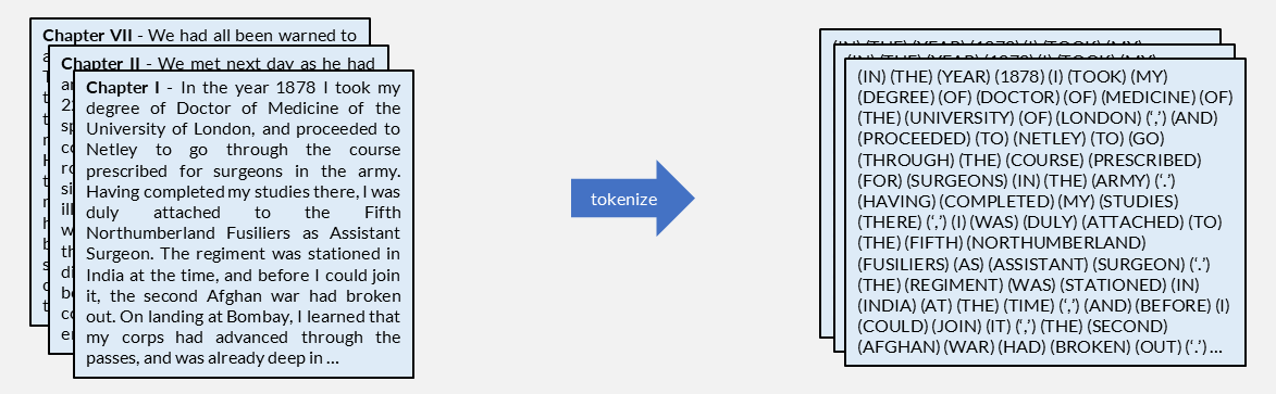
Figure 4:Tokenization: raw text split into individual word-level tokens.
Lemmatization and Stemming
The previous subsection established that retrieval models treat each token as an independent symbol: “cat” and “cats” are unrelated unless we normalize them to the same form. The goal of this pipeline stage is to reduce surface variation so that semantically equivalent word forms map to a single canonical token in the vocabulary.
Two approaches exist:
Stemming applies rule-based suffix stripping to produce a common pseudo-stem. The stem is not necessarily a real word (e.g., “computing”, “computation”, “computer” all reduce to “comput”). Stemming is fast, requires no dictionary, and works well enough for most retrieval tasks. Its errors go in both directions: it can merge unrelated words (“universal” and “university” both stem to “univers”) or fail to merge related ones (“alumnus” and “alumni” remain distinct).
Lemmatization uses a dictionary or morphological analysis to map each word to its actual root form (the lemma). “Better” maps to “good”, “went” maps to “go”. This produces more accurate results but requires language-specific resources and is computationally more expensive. Modern NLP libraries like spaCy provide lemmatization out of the box.
For classical text retrieval, stemming is the standard choice due to its speed and simplicity. The most widely used stemmer for English is the Porter Algorithm, which we examine next.
The Porter Algorithm
The most well-known rule-based stemmer for English is the Porter Algorithm (1980); see An Algorithm for Suffix Stripping in the Further Reading section of the chapter summary. It applies an ordered sequence of suffix-stripping rules to produce a shared pseudo-stem. For the retrieval pipeline, the important result is that related forms map to the same vocabulary term; the exact rule sequence is secondary.
Consider these examples:
| Input | Porter stem | True root |
|---|---|---|
| “computing”, “computation”, “computer” | comput | compute |
| “retrieval”, “retrieving”, “retrieved” | retriev | retrieve |
| “generalization”, “generalizing” | general | generalize |
| “relational” | relat | relate |
| “agreed”, “agreeable” | agre | agree |
The stems “comput”, “retriev”, and “agre” are not dictionary words. They exist only to ensure that related forms map to the same token during indexing. When a user queries “computation”, the system stems it to “comput” and matches documents containing “computing” or “computer” because those were also stemmed to “comput”.
This approach is fast (roughly 60 rules in about 400 lines of code), requires no dictionary, and works well enough for most English retrieval tasks. However, it is purely mechanical and makes errors in both directions: over-stemming merges words that should remain distinct (“operate” and “operating” correctly merge, but “operation” and “operational” may conflate with “opera”), while under-stemming fails to merge irregular forms (“be”, “was”, “been” remain three separate tokens).
Vocabulary
After tokenization and stemming, we have a set of normalized tokens across the entire collection. The vocabulary is the complete set of distinct terms that appear at least once. Each term becomes a dimension in the feature space used for retrieval. But not all terms are equally useful.
Stop Words
Many terms are grammatically necessary but carry no content. The article “the” appears in virtually every English document but tells us nothing about what a document is about. A search for “the” would return the entire collection, unable to differentiate between relevant and non-relevant results. Figure 5 shows that the 50 most frequent terms in a news corpus account for roughly one-third of all occurrences and appear in over 60% of documents.
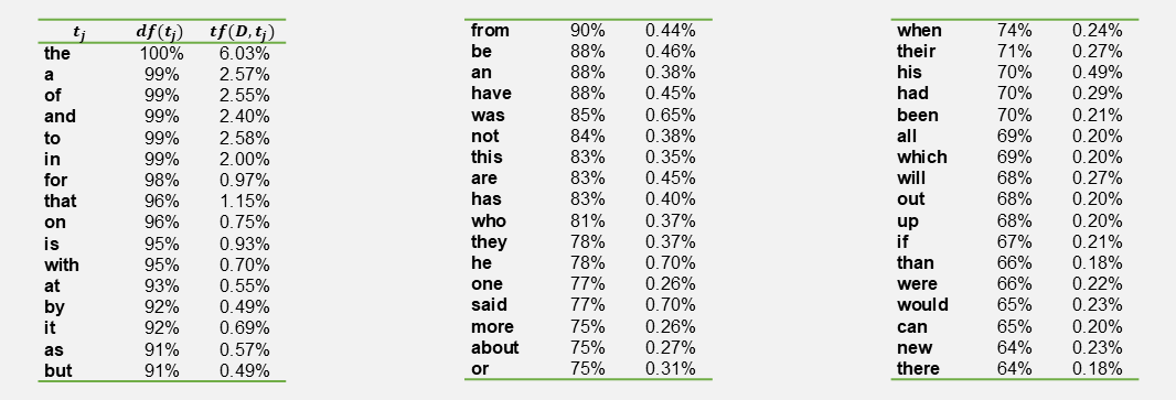
Figure 5:Document frequency and collection term frequency for the 50 most frequent terms in a news corpus (~20,000 documents).
Stop word lists for most languages are readily available, for example on Kaggle (stop words in 28 languages). However, eliminating stop words entirely creates problems. Consider the search for “it”: if we remove this term, we lose the ability to find IT books or the novel “It” by Stephen King. The modern approach retains all terms but assigns them different weights based on their discriminating power.
Zipf’s Law
The distribution of term frequencies follows a remarkably regular pattern. Let be the total number of token occurrences in the collection and the number of distinct terms. If we rank terms by decreasing frequency, Zipf’s law states that the probability of encountering the term at rank is:
The constant depends only on the vocabulary size:
In other words, a few terms dominate the collection while the vast majority are rare.
For a collection with terms, ; with , . The practical implication is shown in Figure 6: terms fall into three zones. The most frequent terms (above the upper cut-off) appear everywhere and cannot discriminate. The rarest terms (below the lower cut-off) are highly specific but unlikely to occur in queries, making them less useful despite their discriminating potential. The terms most useful for distinguishing relevant from non-relevant documents lie in between.
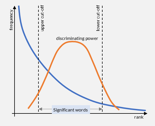
Figure 6:Zipf’s law and term discrimination: the most useful terms for retrieval fall between the frequency extremes.
Term Discrimination and IDF
The intuition behind term weighting is straightforward: imagine removing a single term from every document in the collection. If documents suddenly become harder to tell apart, that term was helping to discriminate between them. Conversely, removing a term that appears everywhere (like “the”) changes nothing. Terms that appear in a moderate number of documents have the highest discriminating power, as confirmed empirically in Figure 7.
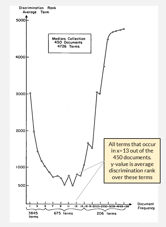
Figure 7:Discrimination rank vs. document frequency in the Medlars collection (450 documents). Terms occurring in 9-12 documents have the highest discrimination rank. Source: Salton, Wong & Yang (1975).
Karen Spärck Jones (1972) captured this intuition in a single formula called the inverse document frequency (IDF); see A Statistical Interpretation of Term Specificity and Its Application in Retrieval in the Further Reading section of the chapter summary. It builds on one statistic: the document frequency , which counts how many documents contain term at least once. IDF then weights terms inversely to their commonness:
IDF provides the weighting mechanism we need: common terms get low weights, rare terms get high weights. Combined with term frequency, it produces the tf·idf weighting that we will use for some of the retrieval models in the next sections. Figure 8 compares IDF weights with empirical discrimination power, confirming that IDF closely approximates the true discriminating value of terms.
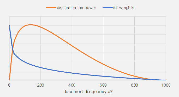
Figure 8:IDF weights closely track empirical discrimination power as a function of document frequency (N = 1,000).
Document Representation
With the vocabulary established and each term assigned an IDF weight, we can now represent documents as vectors. Each document becomes a point in an -dimensional space where is the vocabulary size and each dimension corresponds to one term. Figure 9 shows this process: tokenized text is stemmed, stop words are removed, and the remaining terms are counted to produce per-document frequency vectors.
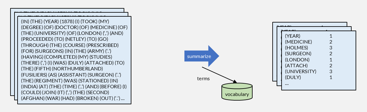
Figure 9:From tokenized text to term-frequency vectors: stem, remove stop words, count occurrences per document.
Set-of-Words and Bag-of-Words
Let be the -th document in a collection of documents. The feature representation is a vector where component describes how term occurs in document . We use to denote the number of occurrences of term in document .
The simplest option is the set-of-words model: for each term, record only whether it is present (1) or absent (0). A document mentioning “cat” three times looks identical to one mentioning it once:
A richer option is the bag-of-words model: record how many times each term appears. A document mentioning “cat” five times is represented differently from one mentioning it once:
Both models ignore term proximity and order. A document containing “New York” is represented the same way as one containing “York New”. Despite this limitation, these representations work remarkably well because the presence and frequency of specific terms are strong signals of relevance.
TF·IDF Weighting
The bag-of-words model treats all terms equally: a document with 10 occurrences of “the” scores the same as one with 10 occurrences of “algorithm”. By combining term frequency with IDF, we produce weighted vectors where informative terms contribute more:
Sparsity
In practice, a vocabulary can include millions of terms. However, most documents contain only a few hundred or thousand unique terms. The feature vectors are therefore sparsely populated: the vast majority of components are zero. Efficient storage methods like the inverted file exploit this sparsity by recording only the non-zero entries. During retrieval, the system only needs to consider documents that share at least one term with the query.