Evaluating Ranked Results - Multimedia Retrieval

Precision and recall treat a result set as a bag: a document is either in the set or not, and the metrics do not change if the order is shuffled. A ranked retrieval system does more than decide which documents to return; it decides which ones to show first. A user who reads from the top and stops after five items gets a very different experience depending on whether the relevant books are at ranks 1 and 2 or at ranks 16 and 18. Evaluation must account for position, not only membership.

Recall the first five positions from Designing a Retrieval Benchmark:

Rank	System A result	Useful?	System B result	Useful?
1	Computer Organization and Design	yes	Database Systems: The Complete Book	yes
2	Operating System Concepts	yes	Pattern Recognition and Machine Learning	yes
3	The Handmaid’s Tale	no	Introduction to Algorithms	yes
4	Narrative of the Life of Frederick Douglass	no	On the Origin of Species	no
5	Towards a New Architecture	no	Introduction to the Theory of Computation	yes

System A retrieves 25 books total (12 of 15 relevant); System B retrieves 8 (6 of 15 relevant). The set-based precision numbers from Precision and Recall already showed that B is more precise overall, but ranking adds a second dimension: how quickly does the user reach useful material? System A places two relevant books at the top, then three misses; System B delivers four of five.

Precision at Rank k¶

The simplest rank-aware metric evaluates only the first $k$ positions. Precision at rank $k$ counts how many of the top- $k$ documents are relevant, ignoring everything below.

$P@k$ answers one practical question: if the user reads only the first $k$ items, what proportion is useful? It does not require knowing how many relevant documents exist in the collection, which makes it easy to compute and interpret. It also does not penalize a system for missing relevant documents below rank $k$ : a system that places one relevant book at rank 1 and nothing else achieves $P@1 = 1.0$ regardless of how many relevant books it missed.

Example: P@k for System A and B

$k$	$P@k$ (A)	$P@k$ (B)
3	2/3 = 66.7%	3/3 = 100%
5	2/5 = 40.0%	4/5 = 80.0%
10	5/10 = 50.0%	6/10 = 60.0%*

*System B returns only 8 documents. Positions 9 and 10 are empty, counted as non-relevant.

System B dominates at every cutoff. A student who reads the first five results gets four useful books from B but only two from A. $P@k$ captures this user experience directly.

Reciprocal Rank and MRR¶

Some information needs have a single correct answer, or the user is satisfied as soon as one relevant result appears. A library patron asking “Who wrote Dracula?” needs exactly one fact; seeing it at rank 1 is ideal, at rank 20 is frustrating. The reciprocal rank captures this notion.

$RR = 1$ when the first result is relevant; $RR = 0.5$ when the first relevant result is at rank 2; $RR \to 0$ as the relevant document is pushed further down. If no relevant document appears in the result list at all, $RR = 0$ .

Example: MRR for fact lookups

MRR is best demonstrated on fact-lookup queries where exactly one answer exists. Suppose four students each ask the library catalogue a different question, and both systems return a ranked list. The only thing that matters is how far down the student must scroll to find the answer:

Query	Answer	System A: rank	$RR_A$	System B: rank	$RR_B$
“Who wrote Dracula?”	Dracula	1	1.000	3	0.333
“A book on operating system design?”	Operating System Concepts	4	0.250	1	1.000
“A nineteenth-century Russian novel?”	Crime and Punishment	6	0.167	2	0.500
“A dystopian novel by Atwood?”	The Handmaid’s Tale	2	0.500	5	0.200

MRR_A = \frac{1.000 + 0.250 + 0.167 + 0.500}{4} = 0.479

(3)

MRR_B = \frac{0.333 + 1.000 + 0.500 + 0.200}{4} = 0.508

(4)

Neither system dominates: A answers one query instantly ( $RR = 1$ ) but buries the Russian novel at rank 6, while B also has one perfect answer but pushes the Atwood question to rank 5. The averages are close, which tells us the two systems surface first answers at comparable speed overall despite different per-query strengths.

MRR is widely used in question answering and known-item search, where one good answer suffices. It ignores what happens after the first relevant document: a system that places five relevant books at ranks 1 through 5 scores the same $RR = 1$ as one that places a single relevant book at rank 1 and nothing else. For needs where multiple relevant documents matter, as in our CS-foundations example with 15 relevant books, MRR is the wrong tool.

The Precision-Recall Curve¶

$P@k$ evaluates one fixed cutoff. A more complete picture plots precision against recall at every rank where a relevant document appears. As the system returns more documents, recall increases (more relevant documents are found) and precision typically decreases (more non-relevant documents accumulate). Plotting precision against recall produces the precision-recall curve.

At each rank $i$ in the result list, define:

P_i = \frac{|\{d_1, \ldots, d_i\} ∩ \text{Rel}|}{i} \qquad R_i = \frac{|\{d_1, \ldots, d_i\} ∩ \text{Rel}|}{|\text{Rel}|}

(5)

A point $(R_i, P_i)$ is recorded only at ranks where a relevant document is retrieved: those are the only ranks where recall changes. Between two relevant documents, recall stays constant while precision drops (the denominator $i$ grows with no new relevant hit), so these in-between ranks do not add new curve points.

Example: Precision-Recall curve for System A

The relevant documents in System A’s ranking appear at ranks 1, 2, 6, 7, 9, 12, 13, 16, 18, 21, 23, and 25. At each of those positions:

Rank	Relevant found	$P_i$	$R_i$
1	1	1/1 = 1.000	1/15 = 0.067
2	2	2/2 = 1.000	2/15 = 0.133
6	3	3/6 = 0.500	3/15 = 0.200
7	4	4/7 = 0.571	4/15 = 0.267
9	5	5/9 = 0.556	5/15 = 0.333
12	6	6/12 = 0.500	6/15 = 0.400
13	7	7/13 = 0.538	7/15 = 0.467
16	8	8/16 = 0.500	8/15 = 0.533
18	9	9/18 = 0.500	9/15 = 0.600
21	10	10/21 = 0.476	10/15 = 0.667
23	11	11/23 = 0.478	11/15 = 0.733
25	12	12/25 = 0.480	12/15 = 0.800

The curve starts at $(0.067, 1.0)$ and ends at $(0.800, 0.480)$ . After rank 2, three consecutive non-relevant books push precision down before the next relevant book at rank 6 lifts it back to 0.5. The curve never reaches recall 1.0 because System A misses 3 of the 15 relevant books.

Reading the Curve¶

Figure 1 annotates the key regions of a precision-recall curve. The upper-left corner (high precision, low recall) is where a fact-checker operates: a short, clean result list with few mistakes. The lower-right corner (high recall, low precision) is where a patent lawyer operates: an exhaustive search that tolerates noise to avoid missing anything. The diagonal arrow labelled “system efficiency” points toward the ideal corner $(1, 1)$ : the closer a curve pushes toward that point, the better the system balances both goals simultaneously.

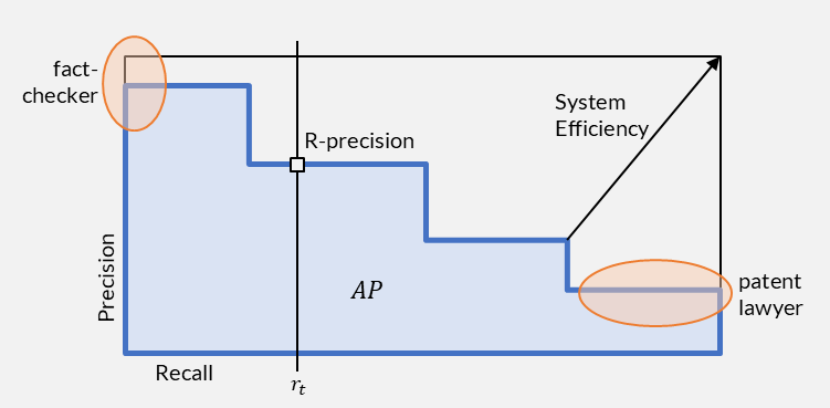
Figure 1:Precision-recall curve with key evaluation landmarks: the shaded area is Average Precision (AP), R-precision marks the point where the number of results equals the number of relevant documents, and the two user profiles illustrate the trade-off between precision-oriented and recall-oriented search.

The shaded area under the curve represents Average Precision (AP), which the next subsection defines formally. The figure marks R-precision at rank $R$ , where $R$ is the number of relevant documents. At this cutoff, precision and recall are numerically equal because both divide the number of relevant documents retrieved in the first $R$ positions by $R$ .

Interpolation for Cross-System Comparison¶

The 12 points in the table above form a smooth, largely decreasing scatter for one system and one need. The need for interpolation arises when we want to compare two systems or average curves across multiple needs: each system produces points at different recall levels, so we cannot directly subtract or average their precisions. Interpolation defines precision at any recall level $r$ as the maximum precision achieved at any recall level $r' \geq r$ :

P_{\text{interp}}(r) = \max_{r' \geq r} P(r')

(6)

This produces a non-increasing step function evaluated at standard recall levels (0, 0.1, 0.2, ..., 1.0). Two systems evaluated on the same 11 recall points can be compared point by point or averaged across queries. For System A, interpolated precision at recall 0 is 1.0 (the best precision it ever achieves), while at recall 0.9 and 1.0 it is 0 (the system never reaches those recall levels).

R-Precision¶

R-precision links precision to recall through a single number. If the collection contains $R$ relevant documents for a need, R-precision is the precision after exactly $R$ documents have been retrieved.

\text{R-Prec} = P@R = \frac{|\{D_1, \ldots, D_R\} ∩ \text{Rel}|}{R}

(7)

A perfect system would place all $R$ relevant documents in the first $R$ positions, achieving R-precision of 1.0. The measure adjusts itself to the difficulty of the need: a need with 15 relevant documents (our CS-foundations example) evaluates at cutoff 15, while a need with 2 relevant documents evaluates at cutoff 2.

R-precision is simple and self-adjusting, but it reduces an entire ranking to one point. The metrics that follow evaluate the full curve.

Average Precision¶

Average precision (AP) collapses the precision-recall curve into a single number. Geometrically, it approximates the area under the precision-recall curve: the shaded region in Figure 1. A system whose curve stays high across all recall levels has a large area and a high AP; one whose precision collapses early has a small area and a low AP.

The computation is straightforward: at each rank where a relevant document appears, record the precision at that rank. Then take the mean of those values, using the total number of relevant documents in the collection as the divisor.

Dividing by $|\text{Rel}|$ rather than by the number of relevant documents actually found means that missed documents contribute implicit zeros: they never appear in the ranking, so they add nothing to the numerator, but the denominator still counts them. This is what makes AP sensitive to recall, not only to precision at the top.

AP uses the raw (non-interpolated) precision values. Interpolation serves a different purpose: it defines precision at arbitrary recall levels so that curves from different systems can be compared point by point or averaged. AP does not require that step because it sums only at the fixed rank positions where relevant documents actually occur.

Example: Average Precision for System A and B

System A finds 12 of 15 relevant documents. The precision at each relevant rank:

AP_A = \frac{1}{15}\left(\frac{1}{1} + \frac{2}{2} + \frac{3}{6} + \frac{4}{7} + \frac{5}{9} + \frac{6}{12} + \frac{7}{13} + \frac{8}{16} + \frac{9}{18} + \frac{10}{21} + \frac{11}{23} + \frac{12}{25}\right) = 0.473

(11)

The three relevant books that System A missed (ranks would be needed beyond 25, or they were never retrieved) each contribute 0 to the sum, pulling the average down.

System B finds 6 of 15 relevant documents, all placed high:

AP_B = \frac{1}{15}\left(\frac{1}{1} + \frac{2}{2} + \frac{3}{3} + \frac{4}{5} + \frac{5}{6} + \frac{6}{8}\right) = 0.359

(12)

System B’s precisions at the positions where it finds relevant documents are higher (it averages 0.897 over its 6 hits vs. A’s 0.592 over its 12 hits), but it misses 9 of 15 relevant books. Those 9 zeros in the denominator dominate: $AP_B < AP_A$ .

AP rewards both placing relevant documents high (each precision term is larger when fewer non-relevant documents precede it) and finding more relevant documents (more terms contribute to the sum). This makes it the single best summary of a ranking for a given need: unlike $P@k$ it accounts for the full list, and unlike MRR it values every relevant document, not only the first.

Mean Average Precision¶

Evaluating a system on one need gives one AP value. A benchmark with multiple needs produces an AP per need, and mean average precision (MAP) averages them.

MAP = \frac{1}{|\mathbb{Q}|}\sum_{i=1}^{|\mathbb{Q}|} AP_i

(13)

MAP is a macro-average: each need contributes equally regardless of how many relevant documents it contains. This is the same averaging strategy discussed in Precision and Recall, and the same caveats apply: a need with one relevant document has as much influence on MAP as a need with fifteen.

Example: MAP across four needs

Using the four needs from our library example:

Need	Relevant	$AP_A$	$AP_B$
CS foundations	15	0.473	0.359
Stage plays	5	0.587	0.600
Atwood books	2	0.833	1.000
Russian novels	1	0.000	1.000

MAP_A = \frac{0.473 + 0.587 + 0.833 + 0.000}{4} = 0.473

(14)

MAP_B = \frac{0.359 + 0.600 + 1.000 + 1.000}{4} = 0.740

(15)

System B wins on MAP despite finding far fewer relevant documents on the largest need. Two factors combine: B has perfect AP on two smaller needs, while A’s zero on Russian novels costs 0.25 in the average, and A also fails to find one of the five plays in its stage-plays run.

MAP is the standard primary metric in TREC and most retrieval benchmarks. A single MAP value summarizes an entire system’s behaviour across all evaluated needs. When two systems are compared, a paired test (such as a paired $t$ -test or Wilcoxon signed-rank test) on the per-need AP values determines whether the difference is statistically significant, not just the result of a few easy or hard queries.

Choosing a Metric¶

Each metric answers a different question about the ranking:

Metric	Question it answers	Sensitive to
$P@k$	How clean are the first $k$ results?	Precision at a fixed cutoff
$MRR$	How quickly does the user find one good result?	Position of the first relevant document
$\text{R-Prec}$	How well does the system fill the first $R$ slots?	Balance of precision and recall at a natural cutoff
$AP$	How good is the overall ranking for one need?	Both precision and recall, position-weighted
$MAP$	How good is the system across many needs?	Per-need AP, macro-averaged

$P@k$ and MRR suit settings where users inspect only the top few results: web search, question answering, voice assistants. AP and MAP suit settings where the full ranking matters: patent search, systematic reviews, benchmark comparisons. R-precision provides a single summary that adjusts to the number of relevant documents per need.

All of these metrics treat relevance as binary: a document is relevant or it is not. The next section relaxes this assumption, introducing graded relevance where some documents are more useful than others, and metrics that reward a system for placing highly relevant documents above marginally relevant ones.