Evaluating Text Classifiers
Retrieval systems do not exist in isolation. A search engine for images relies on classifiers that detect faces, identify objects, or assign scene categories before any query arrives. An audio retrieval system uses a classifier to segment speech from music. A filtering stage in a retrieval pipeline decides “does this candidate pass the criteria?”: a binary classification decision embedded inside retrieval. These classifiers are components of the retrieval pipeline, and they need their own evaluation. The confusion matrix and its metrics appear every time a system makes a binary or multiclass decision, whether that decision is the final answer or a preprocessing step that feeds into ranking.
The underlying evaluation question is familiar: how often does the system make the right decision? Precision and recall still apply. What changes is the framing. There is no “retrieved set” to measure against a collection; instead, the system assigns exactly one label to each item in a test set, and we compare those predictions against ground-truth labels. Three properties make classification evaluation distinct from retrieval evaluation:
No ranking. The system outputs a label, not a position. There is no notion of “rank 3 is better than rank 10”.
Prevalence matters. The proportion of positive items in the test set affects how we interpret every metric. A rare disease affects 1% of patients; a common spam folder holds 40% junk.
Error costs are often asymmetric. A false positive in spam filtering deletes a legitimate email; a false negative lets spam through. These are not equally bad.
The Confusion Matrix
The confusion matrix organizes every prediction the system made into a table for binary classification. Figure 1 shows this arrangement. Each item in the test set falls into exactly one cell, depending on the system’s prediction and the true label.
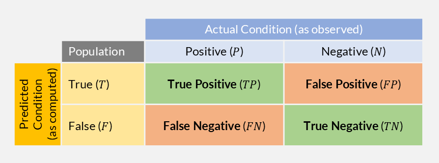
Figure 1:The binary confusion matrix. Rows represent predictions, columns represent actual conditions. Green cells are correct predictions; orange cells are errors.
The row sums give the number of items the system labelled positive () and negative (). The column sums give the actual counts: positive items and negative items in the test set. The total population is .
From these four counts, we derive the same metrics introduced for retrieval, plus several that become important only in classification:
Precision and recall are identical to the retrieval definitions from Precision and Recall, just viewed from a different angle: “retrieved” becomes “predicted positive”, and “relevant” becomes “actually positive”. Specificity is new; in retrieval we called its complement “fallout” (). Accuracy had no retrieval equivalent because retrieval operates on a ranked list, not a fixed yes/no decision for every item.
Figure 2 summarizes how the four outcome counts produce the classification metrics and their complementary rates.
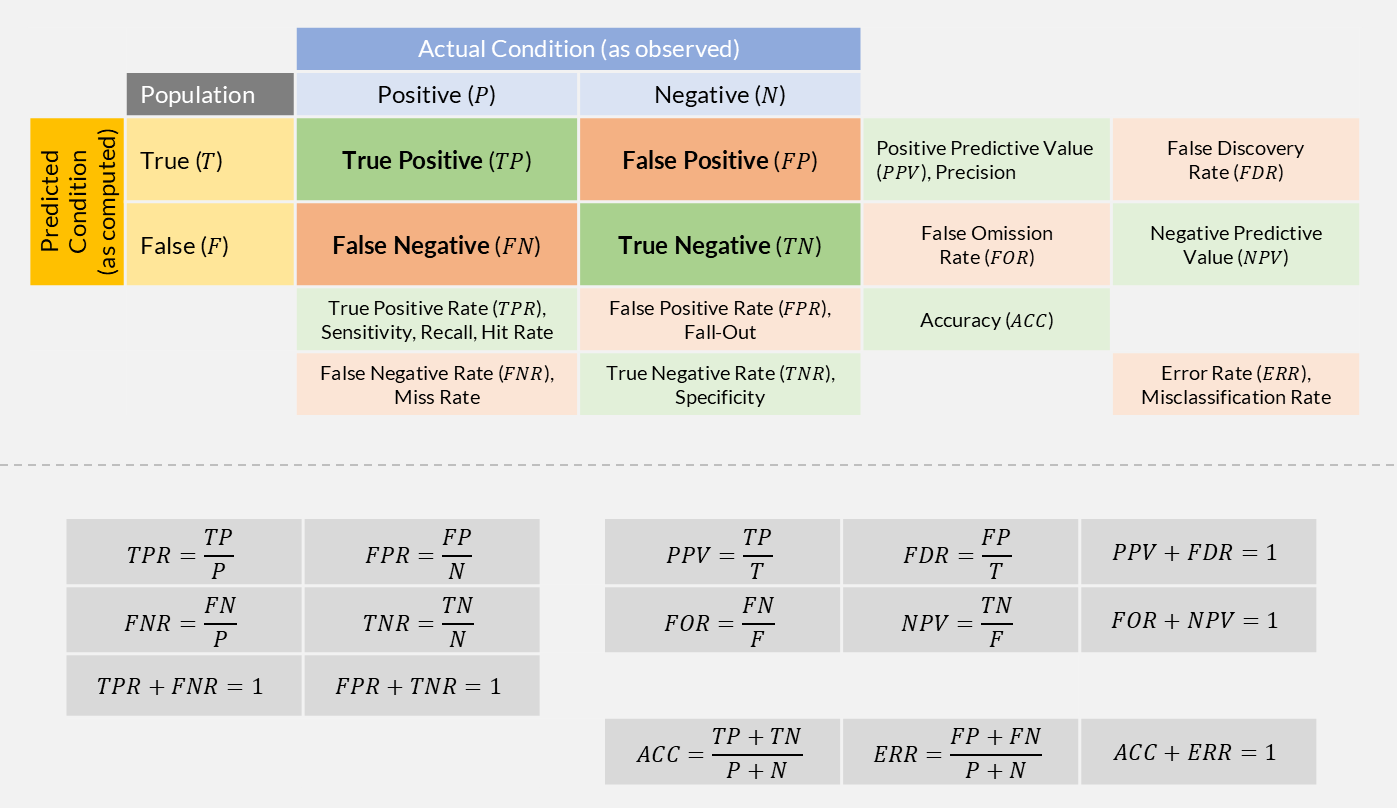
Figure 2:The confusion matrix and its derived metrics. Column-normalized rates (TPR, FPR, FNR, TNR), row-normalized predictive values (PPV, NPV), and overall accuracy, with all complementary pairs summing to one.
Example: Spam Filtering
A university email server processes 1000 messages in one day. Of these, 400 are spam () and 600 are legitimate (). The spam filter makes the following decisions:
| Actual Spam (400) | Actual Legitimate (600) | |
|---|---|---|
| Predicted Spam | TP = 360 | FP = 30 |
| Predicted Legitimate | FN = 40 | TN = 570 |
All four numbers look healthy: the filter catches 90% of spam, and 92% of what it flags is genuinely spam. But consider the 30 false positives: those are 30 legitimate emails moved to the junk folder. If one of them is an acceptance letter for a grant proposal, the cost of that single FP dwarfs the annoyance of 40 spam messages reaching the inbox.
When Accuracy Misleads
Accuracy counts all correct decisions equally. When the two classes are roughly balanced (as in the spam example with 400 vs. 600), accuracy gives a fair summary. When one class dominates, accuracy becomes misleading.
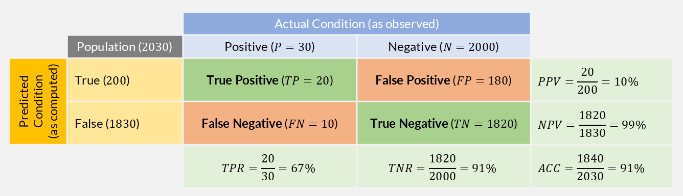
Figure 3:Confusion matrix for an imbalanced dataset (, ). High accuracy (91%) masks low precision (10%) and moderate recall (67%).
Consider a screening test for a rare disease. In a population of 2030 people, 30 have the disease () and 2000 do not (). Figure 3 shows the test outcomes: , , , .
The problem is prevalence: only of the population is positive. With so few positives, even a small false-positive rate () produces many more false positives than true positives in absolute terms. Accuracy is dominated by the 2000 true negatives and hides the fact that the test is nearly useless for confirming the disease.
Asymmetric Error Costs
The spam and screening examples already show that FP and FN carry different costs. A third scenario makes this even starker: biometric face unlock on a smartphone.
The system decides whether the face in front of the camera matches the phone’s owner. Two errors are possible:
False Positive: an impostor’s face is accepted. The phone unlocks for a stranger. This is a security breach.
False Negative: the owner’s face is rejected. The owner must retry or use a PIN. This is a minor inconvenience.
The costs are radically different: a single FP compromises all data on the device, while a FN costs five seconds. The system must therefore achieve an extremely low false-positive rate (FPR), even if this means a noticeable false-negative rate (FNR).
The choice of which error to minimize is not a mathematical question; it is a design decision that precedes evaluation. The metrics merely reveal whether the system meets the requirement. In the next section, we explore how moving a decision threshold trades FPR against FNR continuously, and how ROC curves visualize this trade-off.
Multiclass Classification
Binary classification assigns one of two labels. Many tasks assign one of labels: an image classifier distinguishes “indoor”, “outdoor”, and “portrait”; an AI assistant routes user queries to the correct handler. The confusion matrix generalizes to a table where rows are predicted classes and columns are actual classes.
Per-Class Metrics via One-vs-Rest
To compute precision, recall, and specificity for one class, collapse the matrix into a binary view: “belongs to class ” vs. “does not belong to class ”. Figure 5 shows this collapse for two classes from the intent-routing example.
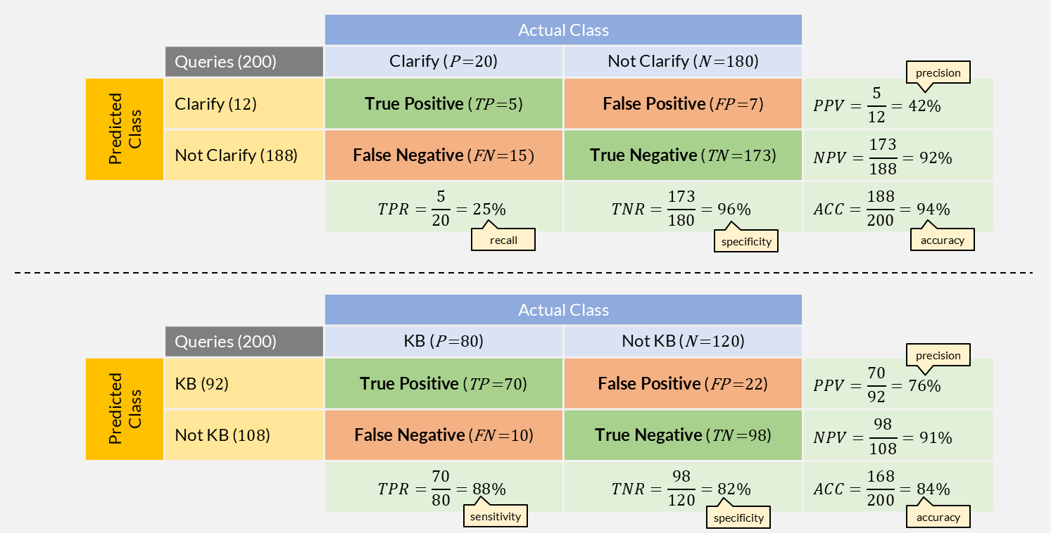
Figure 5:One-vs-rest collapse of the intent-routing confusion matrix for the clarify class (top) and the knowledge_base class (bottom), with derived metrics.
For the clarify class (the rare intent with 20 actual queries), the system correctly identifies only one in four queries that actually need clarification. Most of the rest (12 out of 15 missed) get misrouted to knowledge_base, where the system attempts to answer a question it does not understand. This is the most dangerous failure mode: the user gets a confident but wrong answer instead of a helpful follow-up question.
For the dominant knowledge_base class (80 of 200 queries), the system routes most KB queries correctly (high recall) but also absorbs queries that belong elsewhere (22 false positives), diluting precision. The high recall on the dominant class is what inflates the accuracy of the 4x4 confusion matrix to 76.5%.
Aggregating Across Classes
With classes, we have precision values and recall values. Summarizing them into one number uses the same macro/micro distinction from Precision and Recall:
Macro-averaging computes the metric per class, then takes the arithmetic mean:
Each class contributes equally, regardless of size. For our intent router:
| Class | Precision | Recall |
|---|---|---|
knowledge_base | 0.761 | 0.875 |
web_search | 0.800 | 0.800 |
calculator | 0.833 | 0.750 |
clarify | 0.417 | 0.250 |
Micro-averaging pools TP, FP, and FN across all classes before computing the ratio:
Both denominators equal the total number of queries (200): the precision denominator sums all row totals, the recall denominator sums all column totals, and in a single-label setting these are the same. The numerator is always the sum of the diagonal (correct predictions). So micro-precision, micro-recall, and accuracy all collapse to the same value: diagonal sum divided by total.
This explains why accuracy is the dominant single-number metric in classification: it is the micro-averaged precision and recall. In retrieval, micro-averaging played a secondary role because the macro view (one score per query, then average) better matched evaluation practice. In classification, the micro view is the natural default, and accuracy is its name.
Macro-averaging tells the opposite story. It gives each class equal weight: mean precision drops to 70.3% and mean recall to 66.9%, pulled down by clarify’s dismal 25% recall. If every intent matters equally (and it should, because a misrouted clarify query produces a wrong answer), macro-averaging is the right summary.
All metrics in this section assume a fixed decision: the system outputs a label and we count outcomes. But most classifiers internally produce a continuous score (a probability, a distance, a similarity), and the label emerges only after applying a threshold. Moving that threshold changes the balance between FP and FN. The next section explores this continuous perspective through score distributions, threshold selection, and ROC curves.